Pytorch Study Note 2
Prelude
Last article we talked about basic Tensor unit in PyTorch, the manipulation about it and a light tough on the implementation of linear regression in PyTorch architecture. If you missed the last section, you can review here. As the teaser image suggests, IT IS MATH TIME! Nothing really hard and theoretical, but some basic differentiation techniques will suffice. In this article, we will discuss some very important logics behinds PyTorch that makes it unique and become the favorite of many – the dynamic computation graph and auto gradient. Also, a demo of how to setup logistic regression in PyTorch in practice.
Table of Content
- Computation Graph
- Auto Gradient
- Logistic Regression
Computation Graph
Previously, we have talked about tensors, and in machine learning, tensors operations will are error-prone and complicated to work with. Especially when you have a large deep neural net and each layer is a high-dimensional tensor, the interaction between them can be troublesome.
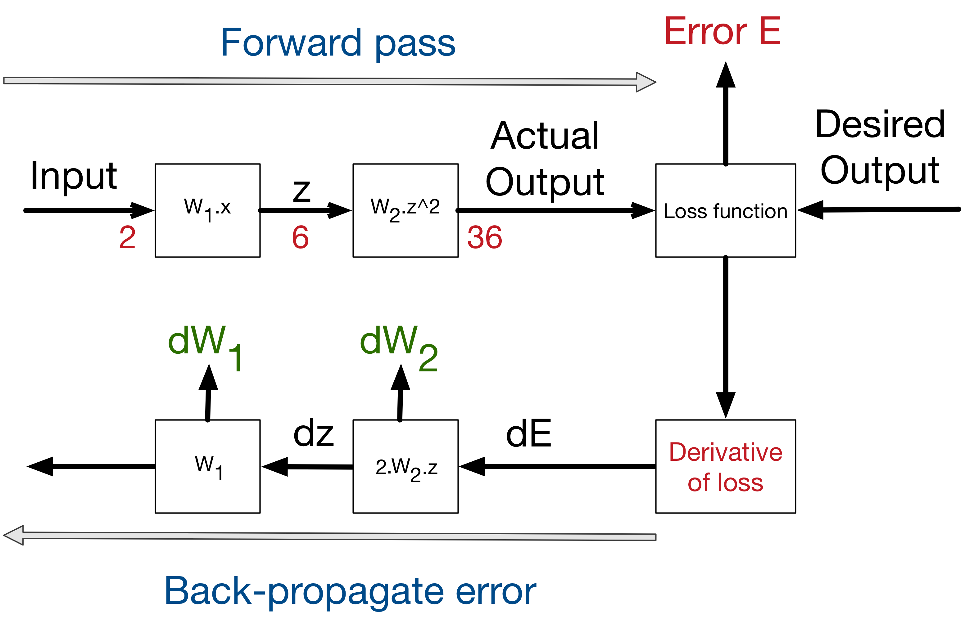
Imagine you have a neural net need for forward propagation, you pass in the value can calculate the value propagation in a chain, you need to link them in a particular way such that the system can automate the process and output your current error; then when you back propagate the gradients and update weights, you reverse the direction of your forward propagation. This is like a ripple, which you hit with forward pass, and feedback with backward propagation. The path forward propagation and backward propagation is finite, just differ in terms of direction.
Computation graph, in this case, is a path, a graph, that clarify and simplify the logic between tensors and layers, and automate the data propagations in between.
From an example
Let’s build a computation graph for
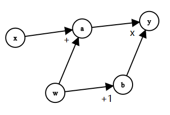
\[y=(x+w)\times (w+1)\]We do it this way:
\[a = x+w\] \[b = w+1\]Then
\[y = a \times b\]And the graph simply looks like this:
Then let’s do back propagation to derive \(\frac{\partial y}{\partial w}\)
By mathematic derivations, we have:
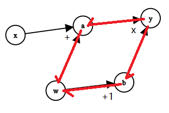
\[\begin{align*} \frac{\partial y}{\partial w} &= \frac{\partial y}{\partial a} \times \frac{\partial a}{\partial w} + \frac{\partial y}{\partial b} \times \frac{\partial b}{\partial w} \\\\ & = b \times 1 + a \times 1 \\\\ & = (w+1) + (w + x) \\\\ & = 2w + x + 1 \\\\ \end{align*}\]With w = 1, x = 2, we have \(y = (1+1)\times (1+2) = 6\), and \(\frac{\partial y}{\partial w} = 2\times 1+1+1 = 5\)
The derivative of y with respect to w, is simply finding all the path from y to w in the graph, and then sum them together. Indicated in red below:
Let’s verify this with code as well:
w = torch.tensor([1.], requires_grad=True)
x = torch.tensor([2.], requires_grad=True)

a = torch.add(w, x)
b = torch.add(w, 1)
y = torch.mul(a, b)

y.backward()
print(w.grad)   # tensor([5.])
Properties
Now we know what a computation graph is, and we can carry on talk about its properties in PyTorch:
-
is_leaf:Remember there is a parameter in
Torch.Tensorcalledis_leaf? You can recap here. Leaf nodes are basically all the nodes that created by user, i.e.wandxin our example. This is very important, since all the propagations are based on our leaf nodes, andis_leafis an indicator telling weather it is a leaf nodeWe can check by this code:
print("is_leaf:\n", w.is_leaf, x.is_leaf, a.is_leaf, b.is_leaf, y.is_leaf)
# is_leaf:
# True True False False False
But why leaf node? I mean why we especially separate those nodes that created by user and those are not? Well PyTorch do this to save memory. Normally, only gradients of leaf nodes are accessed by users. PyTorch is programed especially to save only the leaf node gradients after propagation, but release the memory of non-leaf node gradients.
Let’s check:
print("gradient:\n", w.grad, x.grad, a.grad, b.grad, y.grad)
# gradient:
# tensor([5.]) tensor([2.]) None None None
Well, if you really need to access the gradients in non-leaf gradients, say debugging purpose, you can use
retain_grad()to do so:w = torch.tensor([1.], requires_grad=True) x = torch.tensor([2.], requires_grad=True) a = torch.add(w, x) # we want to keep the gradient in a a.retain_grad() b = torch.add(w, 1) y = torch.mul(a, b) y.backward() print("gradient:\n", w.grad, x.grad, a.grad, b.grad, y.grad) ## gradient of a is preserved # gradient: # tensor([5.]) tensor([2.]) tensor([2.]) None None -
grad_fnRecord how the tensor is calculated i.e. the function to derive the result.
print("grad_fn:\n", w.grad_fn, x.grad_fn, a.grad_fn, b.grad_fn, y.grad_fn)

#None None <AddBackward0 object at 0x0000029AECF56D08> <AddBackward0 object at 0x0000029AEEFEB248> <MulBackward0 object at 0x0000029AEEFEB748>
You can see that a and b is acquired by summation, and y is acquired by multiplication. This is important for back propagation
Dynamic v.s. Static
Why is PyTorch called ‘Dynamic’ computation graph, while TensorFlow is ‘Static’?
The difference is:
- in TensorFlow, we build graph first, then compute or propagate the value. This is very efficient, but hard for tuning
- in PyTorch, graph and computation went together. This is easing the process of graph changing and tuning
Let’s see what it looks like in above scenario:
# Declare two constants
w = tf.constant(1.)
x = tf.constant(2.)

# build graph
a = tf.add(w, x)
b = tf.add(w, 1)
y = tf.multiply(a, b)

# Propagation not started yet, y is just a node
print(y)
# Tensor("Mul_4:0", shape=(), dtype=float32)

with tf.Session() as sess:
    # computation happens in the session
    print(sess.run(y))
    # 6.0
You can see that in TensorFlow, you have to build the graph structure first, then feed in the value to make it flows, while in PyTorch, again:
w = torch.tensor([1.], requires_grad=True)
x = torch.tensor([2.], requires_grad=True)

a = torch.add(w, x)
b = torch.add(w, 1)
y = torch.mul(a, b)
print(y)    # tensor([6.], grad_fn=<MulBackward0>)
computation takes place once the graph is made immediately
Auto Gradient
AutoGrad stands for ‘Automatic Gradient’, which takes the gradient(or derivative) for each variable nodes in the computation graph. I cannot tell how good this feature is, just imagine the amount of trouble there will be for manually calculate the gradient in each neuron in a deep net 🐱🏍.
Backward()
The mechanism behind PyTorch AutoGrad it that torch.autograd.backward function, in detail:
torch.autograd.backward(tensors,
                        grad_tensors=None,
                        retain_graph=None,
                        create_graph=False)
tensoris the tensor that needed to take gradient. Usually the loss functiongrad_tensorsstands for weighing for multiple gradients. If there are multiple loss function that needed to be calculated, we can set weight between their outcomes.retain_graphAs mentioned earlier, non-leaf node gradients will be released after propagation, so does the computation graph. Set toTruecan save the computation graphcreate_graphcan create computation graph that saved for higher order gradient computation
And previously, we pull the autograd function not by explicitly saying torch.autograd.backward, but executed with this order: y.backward()
Here are some cases that we may encounter in the program:
- About
retain_graphw = torch.tensor([1.], requires_grad=True) x = torch.tensor([2.], requires_grad=True) a = torch.add(w, x) # we want to keep the gradient in a a.retain_grad() b = torch.add(w, 1) y = torch.mul(a, b) y.backward() print(w.grad) y.backward() # RuntimeError: Trying to backward through the graph a second time, .....This will give us an error, since after the first
backward(), the computation graph is released, and the secondbackward()won’t be effective anymoreBut if we set the first
backward()tobackward(retain_graph=True), the program will save the computation graph and come useful for the second propagation - About
grad_tensorsw = torch.tensor([1.], requires_grad=True) x = torch.tensor([2.], requires_grad=True) a = torch.add(w, x) # we want to keep the gradient in a a.retain_grad() b = torch.add(w, 1) y0 = torch.mul(a, b) y1 = torch.add(a, 10) loss = torch.cat([y0,y1], dim=0) loss.backward() # RuntimeError: grad can be implicitly created only for scalar inputsThis gives you an error because our loss function has two parameters and need to balance in between.
We simply add a weight for the gradients to the
grad_tensorsparametergrad_tensors = torch.tensor([1., 1.]) loss.backward(gradient=grad_tensors) print(w.grad) # tensor([6.]) because 5+1 grad_tensors = torch.tensor([1., 2.]) loss.backward(gradient=grad_tensors) print(w.grad) # tensor([7.]) because 5+1*2
grad()
There is also a commonly used method in autograd: torch.autograd.grad(), this function takes the gradient of certain variable, even higher order derivatives. In detail:
torch.autograd.grad(outputs,
                    inputs,
                    grad_outputs=None,
                    retain-graph=None,
                    create_graph=False)
Those parameters are quite similar to the parameters we had before, I will not elaborate here.
Let’s take a look at few examples:
- Basics
x = torch.tensor([3.], requires_grad=True) y = torch.pow(x, 2) # y=x^2 # First derivative grad_1 = torch.autograd.grad(y, x, create_graph=True) # We must have computation graph saved here # grad_1 = dy/dx = 2x print(grad_1) # (tensor([6.], grad_fn=<MulBackward0>),) # This is a tuple output, and we only need the first component grad_1[0] # when taking second derivative # Second derivative grad_2 = torch.autograd.grad(grad_1[0], x) # grad_2 = d(dy/dx) /dx = 2 print(grad_2) # (tensor([2.]),) - Taking Gradients for Multiple x(s) and y(s)
 x1 = torch.tensor(1.0,requires_grad = True)
 x2 = torch.tensor(2.0,requires_grad = True)
 # x1, x2 needed to take gradients

 y1 = x1*x2
 y2 = x1+x2

 # Allowing more than one x here
 (dy1_dx1,dy1_dx2) = torch.autograd.grad(outputs=y1,inputs = [x1,x2],retain_graph = True)
 # dy1/dx1 = x2
 # dy1/dx2 = x1
 print(dy1_dx1,dy1_dx2)
 # tensor(2.) tensor(1.)

 # For more than one y, we sum over y(s)
 (dy12_dx1,dy12_dx2) = torch.autograd.grad(outputs=[y1,y2],inputs = [x1,x2])
 # dy2/dx1 = 1
 # dy2/dx2 = 1
 # dy12_dx1 = dy1/dx1+dy2/dx1
 # dy12_dx2 = dy1/dx2+dy2/dx2
 print(dy12_dx1,dy12_dx2)        # tensor(3.) tensor(2.)
There are several important matters to be addressed for PyTorch Autograd system
- Gradient will not be released once
retain_graph = Truew = torch.tensor([1.], requires_grad=True) x = torch.tensor([2.], requires_grad=True) for i in range(4): a = torch.add(w, x) b = torch.add(w, 1) y = torch.mul(a, b) y.backward() print(w.grad) # Result: #tensor([5.]) #tensor([10.]) #tensor([15.]) #tensor([20.])Notice that the gradient for w is accumulated each time, rather than a new gradient. This can be error-prone since each time we want a new adapted gradient when we train a neural net. Therefore, we need to zero out the gradient manually instead:
w = torch.tensor([1.], requires_grad=True) x = torch.tensor([2.], requires_grad=True) for i in range(4): a = torch.add(w, x) b = torch.add(w, 1) y = torch.mul(a, b) y.backward() print(w.grad) w.grad.zero_() # Result: #tensor([5.]) #tensor([5.]) #tensor([5.]) #tensor([5.]) - Nodes depends on leaf nodes will have field
requires_grad=Trueby default From the example we gave previously, since w, x are leaf nodes. When we compute the gradients for w and x, the gradient of a and b will be needed as well for the code to work. We can check with the following code:w = torch.tensor([1.], requires_grad=True) x = torch.tensor([2.], requires_grad=True) a = torch.add(w, x) b = torch.add(w, 1) y = torch.mul(a, b) # y0=(x+w) * (w+1) # dy0 / dw = 5 print(w.requires_grad, a.requires_grad, b.requires_grad) # True, True, True - No in-place operation for leaf node
What is ‘in-place operation’? It mean changing an object without changing its address. This is very basic in python. For example, you have
a=1, then you performa = a+1. We call the firstawitha1=1, the secondawitha2anda2 = a1+1 = 2. In this case,a1anda2are NOT in-place since they have totally different address and values, even though the operation is onadirectly. A in-place operation would bea+=1, where the operation happens directly to the addressais pointing to.a = torch.ones((1,)) print(id(a), a) # 1407221517102 tensor([1.]) # a = a + 1 a = a + torch.ones((1,)) print(id(a), a) # 1407509382238 tensor([2.]) # the two 'a' are not in the same address. This is not a in-place # what about in-place? a = torch.ones((1,)) print(id(a), a) # 2112218352120 tensor([1.]) a += torch.ones((1,)) print(id(a), a) # 2112218352120 tensor([2.])So why we don’t want in-place operation when we calculate the gradient of w in our example(or in general)? Simple because when some calculate involves w, we want to use the original value of w. In-place operation on w will change the value of w, and mess up the gradient value. Therefore, in PyTorch computation graph, in-place operation is prohibited to prevent this error. In the example we use
torch.add(w, 1)rather thanw.add_(1)
Logistic Regression

Model Review
A few review on the logistic regression:
Logistic Regression is linear function to model binary dependent variables
With the following expression:
\[\begin{align*} y &= f(wx+b) \\\\ f(x) &= \frac{1}{1+e^{-x}} \end{align*}\]where f(x) is what we called sigmoid function
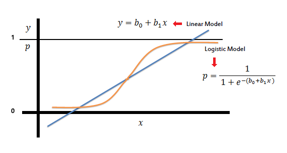
And by binary, we classify the linear values as follows:
\[\text { class }=\left\{\begin{array}{l} 0,0.5>y \\ 1,0.5 \leq y \end{array}\right.\]If you find this regression confusing, I suggest you take through this tutorial to get a better grasp of the model and its properties.
Modeling in PyTorch
Now, enough of the logistic regression, lets train a logistic regression with PyTorch
There are some vital steps for machine learning models:
- Data (Data collection, cleaning, and preprocessing)
- Build Model
- Loss Function (Different loss/Objective for training, then we can take the gradient)
- Optimizer (Optimize the process with some optimizer after acquiring the gradients)
- Iterative Training
Let’s follow this step by step:
- Data Generation
We create artificial data here to experiment the data. We randomly generate two categories of samples (0 or 1), and 100 in each category.
# fixed result torch.manual_seed(1) sample_nums = 100 mean_value = 1.7 bias = 1 n_data = torch.ones(sample_nums, 2) x0 = torch.normal(mean_value*n_data, 1) + bias # category 0, x1, shape=(100,2) y0 = torch.zeros(sample_nums) # category 0,y1, shape=(100,1) x1 = torch.normal(-mean_value*n_data, 1) + bias # category 1,x2, shape=(100,2) y1 = torch.ones(sample_nums) # category 1, y2, shape=(100,1) train_x = torch.cat([x0, x1], 0) train_y = torch.cat([y0, y1], 0) # we concat the data vertically to make a entire dataset - Build Model
There are basically two ways to build our models: sequential and nn.Module. Sequential is easy to start and intuitive, while
nn.Moduleis more computer scientific way, it works as a ‘class’ in python that allows you building more complicated structures. nn.Sequentiallr_net = torch.nn.Sequential( torch.nn.Linear(2, 1), # Linear is a sub-module, it takes input of size 2 and output of size 1 torch.nn.Sigmoid() )nn.Module
class LR(torch.nn.Module): def __init__(self): super(LR, self).__init__() self.features = torch.nn.Linear(2, 1) self.sigmoid = torch.nn.Sigmoid() def forward(self, x): x = self.features(x) x = self.sigmoid(x) return x lr_net = LR() # make a LR object - Loss Function
There will be an article about loss functions in PyTorch in details later. Here we use the binary cross entropy loss, which is common choice for logistic regressions
loss_fn = torch.nn.BCELoss() - Optimizer
There will also be an article about optimizer in PyTorch specifically later. There we use stochastic gradient descendent(SGD), with learning rate of 0.1 and momentum of 0.9
lr = 0.01 optimizer = torch.optim.SGD(lr_net.parameters(), lr=lr, momentum=0.9) - Iterative Training
Now we triggers the training iteratively. It is simply a for loop that repeat a loop over and over again:
forward propagation -> calculate gradient -> back propagation -> update parameters (weights and bias) -> zeroing gradient -> again
  for iteration in range(1000):
    # forward propagation
    y_pred = lr_net(train_x)
    # calculate loss
    loss = loss_fn(y_pred.squeeze(), train_y)
    # back propagation
    loss.backward()
    # update parameters
    optimizer.step()
    # zeroing gradients
    optimizer.zero_grad()
    # graph
    if iteration % 20 == 0:

        mask = y_pred.ge(0.5).float().squeeze()
        # use 0.5 as a threshold
        correct = (mask == train_y).sum()
        # calculate how many are correctly categorized
        acc = correct.item() / train_y.size(0)
        # calculate categorization accuracy

        plt.scatter(x0.data.numpy()[:, 0], x0.data.numpy()[:, 1], c='r', label='class 0')
        # scatter plot for class 0, ground truth
        plt.scatter(x1.data.numpy()[:, 0], x1.data.numpy()[:, 1], c='b', label='class 1')
        # scatter plot for class 1, ground truth

        w0, w1 = lr_net.features.weight[0]
        w0, w1 = float(w0.item()), float(w1.item())
        # get the weights where y' = w0*x0 + w1*x1 + b, and dataset in form (x0, x1) mapped to y'
        # y = sigmoid(y')
        plot_b = float(lr_net.features.bias[0].item())
        # get the bias term b
        plot_x = np.arange(-6, 6, 0.1)
        plot_y = (-w0 * plot_x - plot_b) / w1
        # x2 = (-w0*x1-b)/w1, where y'=0

        plt.xlim(-5, 7)
        plt.ylim(-7, 7)
        plt.plot(plot_x, plot_y)

        plt.title("Iteration: {}\nw0:{:.2f} w1:{:.2f} b: {:.2f} accuracy:{:.2%} loss:{:.4f}".format(iteration, w0, w1, plot_b, acc, loss.data.numpy()))
        plt.legend()

        plt.show()
        plt.pause(0.5)

        if acc > 0.99:
            break
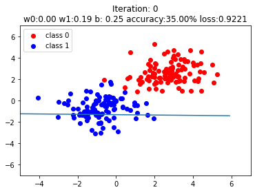

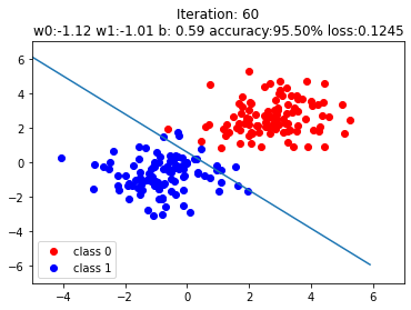
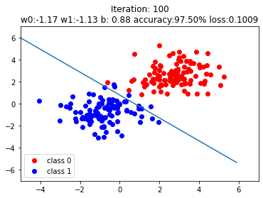
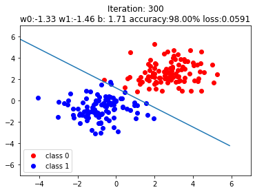
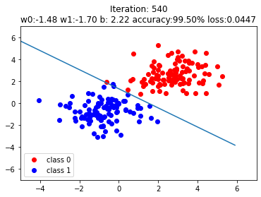
The steps after if iteration % 20 == 0: are not very important, just plots to illustrate the results. The boundary layers are shown on purpose to see how the systems adepts to the data with transition of iterations.
Summary
With the help of computation graph and autograd, we can make simple machine learning models like logistic regression📈. Put in a metaphor of ML to human history, we now get into the stone age, when human has crafted tool🏹 on their right hand and kindle🔥 on their left. This is a small step but significant for building a gigantic PyTorch model in the future.
In the future, we will roughly follow the path we introduced earlier: Data -> Model -> Loss Function -> Optimizer -> Training, and try to explore all the aspects in PyTorch without a miss on the territory🌴.