
Language Model with Neural Net
Introduction:
This project works with word embeddings and making neural networks learn about words. 📖
We could try to match statistics about the words, or we could train a network that takes a sequence of words as input and learns to predict the word that comes next.

Starter code and data
Look at the file raw_sentences.txt.
No , he says now . And what did he do ? The money ‘s there . That was less than a year ago . But he made only the first . There ‘s still time for them to do it . But he should nt have . They have to come down to the people . I do nt know where that is . No , I would nt . Who Will It Be ? And no , I was not the one . You could do a Where are they now ? There ‘s no place like it that I know of . Be here now , and so on . It ‘s not you or him , it ‘s both of you . So it ‘s not going to get in my way . When it ‘s time to go , it ‘s time to go . No one ‘s going to do any of it for us . Well , I want more . Will they make it ? Who to take into school or not take into school ? But it ‘s about to get one just the same . We all have it . So we will be .
It contains the sentences that we are going to analyse These sentences are fairly simple ones and cover a vocabulary of only 250 words.
First, data import
import collections
import pickle
import numpy as np
from tqdm import tqdm
import pylab
use_colab = True
if use_colab:
  from google.colab import drive
import os

TINY = 1e-30
EPS = 1e-4
nax = np.newaxis
if use_colab:
  drive_name = '/content/drive'
  drive.mount(drive_name)
  drive_folder = # your drive folder
  drive_location = drive_name + '/My Drive/' + drive_folder  # Change this to where your files are located
else:
  # set the drive_location variable to whereever the extracted contents are.
  drive_location = os.getcwd()
  # print(drive_location)

data_location = drive_location + '/' + 'data.pk'
PARTIALLY_TRAINED_MODEL = drive_location + '/' + 'partially_trained.pk'
Go to this URL in a browser: ****

Enter your authorization code:
··········
Mounted at /content/drive
We have already extracted the 4-grams from this dataset and divided them into training, validation, and test sets. To inspect this data, run the following:
data = pickle.load(open(data_location, 'rb'))
print(data['vocab'][0])
print(data['train_inputs'][:10])
print(data['train_targets'][:10])
all
[[ 27  25  89]
 [183  43 248]
 [182  31  75]
 [116 246 200]
 [222 189 248]
 [ 41  73  25]
 [241  31 222]
 [222  31 157]
 [ 73  31 220]
 [ 41 191  90]]
[143 116 121 185   5  31  31 143  31  67]
Now data is a Python dict which contains the vocabulary, as well as the inputs and targets for all three splits of the data. data[‘vocab’] is a list of the 250 words in the dictionary; data[‘vocab’][0] is the word with index 0, and so on. data[‘train_inputs’] is a 372,500 x 3 matrix where each row gives the indices of the 3 context words for one of the 372,500 training cases.
data[‘train_targets’] is a vector giving the index of the target word for each training case. The validation and test sets are handled analogously.
Part 1: GLoVE Word Representations
Now, we will implement a simplified version of the GLoVE embedding with the loss defined as
\(L(\{\mathbf{w}_i,b_i\}_{i=1}^V) = \sum_{i,j=1}^V (\mathbf{w}_i^\top\mathbf{w}_j + b_i + b_j - \log X_{ij})^2\).
Note that each word is represented by a d-dimensional vector \(\mathbf{w}_i\) and a scalar bias \(b_i\).
We have provided a few functions for training the embedding:
- calculate_log_co_occurence computes the log co-occurrence matrix of a given corpus
- train_GLoVE runs momentum gradient descent to optimize the embedding
- loss_GLoVE: INPUT - \(V\times d\) matrix \(W\) (collection of \(V\) embedding vectors, each d-dimensional); \(V\times 1\) vector \(\mathbf{b}\) (collection of \(V\) bias terms); \(V \times V\) log co-occurrence matrix. OUTPUT - loss of the GLoVE objective
- grad_GLoVE: INPUT - \(V\times d\) matrix \(W\), \(V\times 1\) vector b, and \(V\times V\) log co-occurrence matrix. OUTPUT - \(V\times d\) matrix grad_W containing the gradient of the loss function w.r.t. \(W\); \(V\times 1\) vector grad_b which is the gradient of the loss function w.r.t. \(\mathbf{b}\).
The math just looks awful huh? Some code will make sense!
vocab_size = 250

def calculate_log_co_occurence(word_data):
  "Compute the log-co-occurence matrix for our data."
  log_co_occurence = np.zeros((vocab_size, vocab_size))
  for input in word_data:
    log_co_occurence[input[0], input[1]] += 1
    log_co_occurence[input[1], input[2]] += 1
    # If we want symmetric co-occurence can also increment for these.
    # Optional: How would you generalize the model if our target co-occurence isn't symmetric?
    log_co_occurence[input[1], input[0]] += 1
    log_co_occurence[input[2], input[1]] += 1
  delta_smoothing = 0.5  # A hyperparameter.  You can play with this if you want.
  log_co_occurence += delta_smoothing  # Add delta so log doesn't break on 0's.
  log_co_occurence = np.log(log_co_occurence)
  return log_co_occurence
log_co_occurence_train = calculate_log_co_occurence(data['train_inputs'])
log_co_occurence_valid = calculate_log_co_occurence(data['valid_inputs'])
calculate the gradient of the loss function w.r.t. the parameters \(W\) and \(\mathbf{b}\). You should vectorize the computation, i.e. not loop over every word.
def loss_GLoVE(W, b, log_co_occurence):
  "Compute the GLoVE loss."
  n,_ = log_co_occurence.shape
  return np.sum((W @ W.T + b @ np.ones([1,n]) + np.ones([n,1])@b.T - log_co_occurence)**2)

def grad_GLoVE(W,  b, log_co_occurence):
  "Return the gradient of GLoVE objective w.r.t W and b."
  "INPUT: W - Vxd; b - Vx1; log_co_occurence: VxV"
  "OUTPUT: grad_W - Vxd; grad_b - Vx1"
  n,_ = log_co_occurence.shape

  grad_W = 4*(W @ W.T + b @ np.ones([1,n]) + np.ones([n,1]) @ b.T - log_co_occurence) @ W
  grad_b = 4*(W @ W.T + b @ np.ones([1,n]) + np.ones([n,1]) @ b.T - log_co_occurence) @ np.ones([n,1])

  return grad_W, grad_b

def train_GLoVE(W, b, log_co_occurence_train, log_co_occurence_valid, n_epochs, do_print=False):
  "Traing W and b according to GLoVE objective."
  n,_ = log_co_occurence_train.shape
  learning_rate = 0.2 / n  # A hyperparameter.  You can play with this if you want.
  for epoch in range(n_epochs):
    grad_W, grad_b = grad_GLoVE(W, b, log_co_occurence_train)
    W -= learning_rate * grad_W
    b -= learning_rate * grad_b
    train_loss, valid_loss = loss_GLoVE(W, b, log_co_occurence_train), loss_GLoVE(W, b, log_co_occurence_valid)
    if do_print:
      print(f"Train Loss: {train_loss}, valid loss: {valid_loss}, grad_norm: {np.sum(grad_w**2)}")
  return W, b, train_loss, valid_loss
Train the GLoVE model for a range of embedding dimensions
np.random.seed(1)
n_epochs = 500  # A hyperparameter.  You can play with this if you want.
# embedding_dims = np.array([1,2,7,10,11,12,15,50,100, 120, 300])  # Play with this
embedding_dims = np.array([1,2,256])
final_train_losses, final_val_losses = [], []  # Store the final losses for graphing
W_final_2d, b_final_2d = None, None
do_print = False  # If you want to see diagnostic information during training
for embedding_dim in tqdm(embedding_dims):
  init_variance = 0.1  # A hyperparameter.  You can play with this if you want.
  W = init_variance * np.random.normal(size=(250, embedding_dim))
  b = init_variance * np.random.normal(size=(250, 1))
  if do_print:
    print(f"Training for embedding dimension: {embedding_dim}")
  W_final, b_final, train_loss, valid_loss = train_GLoVE(W, b, log_co_occurence_train, log_co_occurence_valid, n_epochs, do_print=do_print)
  if embedding_dim == 2:
    # Save a parameter copy if we are training 2d embedding for visualization later
    W_final_2d = W_final
    b_final_2d = b_final
  final_train_losses += [train_loss]
  final_val_losses += [valid_loss]
  if do_print:
    print(f"Final validation loss: {valid_loss}")
100%|██████████| 3/3 [00:11<00:00, 3.85s/it]
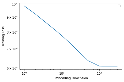
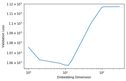
Plot the training and validation losses against the embedding dimension.
Some questions to ask yourself:
- Given the vocabulary size \(V\) and embedding dimensionality \(d\), how many parameters does the GLoVE model have?
\[V\times d + d\]
- Write the gradient of the loss function with respect to one parameter vector \(\mathbf{w}_i\).
\(\frac{\partial L}{\partial w_i} = 2\sum_{j=1, j\neq i}^{V}(w_i^Tw_j + b_i + b_j - \log{X_{ij}})w_j\) \(= 4\sum_{j=1}^{V}(w_i^Tw_j + b_i + b_j - \log{X_{ij}})w_j\)
\(\frac{\partial L}{\partial b_i} = 2\sum_{j=1, j\neq i}^{V}w_i^Tw_j + b_i + b_j - \log{X_{ij}}\) \(= 4\sum_{j=1}^{V}w_i^Tw_j + b_i + b_j - \log{X_{ij}}\)
- Train the model with varying dimensionality \(d\). Which \(d\) leads to optimal validation performance? Why does / doesn’t larger \(d\) always lead to better validation error?
when d = 11, d leads to optimal validation performance with the smallest validation error. This dimentionality indicates a possible encoding of \(2^{11} = 2048\) ways. Model may be over fit if dimension is too large, while underfit if dimension is too small.
Part 2: Network Architecture
-
-
Word embedding weight: \(250\times 16\)
-
Embedded to hidden weight: \(3\times16\times 128\)
-
Hidden to output weight: \(128\times 250\)
-
Hidden bias: \(128\times 1\)
-
Output bias: \(250\times1\)
-
Total: 42522 parameters. The hidden to output weight has the most parameters
-
- A 4-grams model is a model predict the 4th word from 3 previous words. That is, we have 250 vocabularies in total, there is a combination of \(250^4 = 3906250000\) possible non-repeated outcomes.
Part 3: Training the model
There are three classes defined in this part: Params, Activations, Model.
class Params(object):
    """A class representing the trainable parameters of the model. This class has five fields:

           word_embedding_weights, a matrix of size N_V x D, where N_V is the number of words in the vocabulary
                   and D is the embedding dimension.
           embed_to_hid_weights, a matrix of size N_H x 3D, where N_H is the number of hidden units. The first D
                   columns represent connections from the embedding of the first context word, the next D columns
                   for the second context word, and so on.
           hid_bias, a vector of length N_H
           hid_to_output_weights, a matrix of size N_V x N_H
           output_bias, a vector of length N_V"""

    def __init__(self, word_embedding_weights, embed_to_hid_weights, hid_to_output_weights,
                 hid_bias, output_bias):
        self.word_embedding_weights = word_embedding_weights
        self.embed_to_hid_weights = embed_to_hid_weights
        self.hid_to_output_weights = hid_to_output_weights
        self.hid_bias = hid_bias
        self.output_bias = output_bias

    def copy(self):
        return self.__class__(self.word_embedding_weights.copy(), self.embed_to_hid_weights.copy(),
                              self.hid_to_output_weights.copy(), self.hid_bias.copy(), self.output_bias.copy())

    @classmethod
    def zeros(cls, vocab_size, context_len, embedding_dim, num_hid):
        """A constructor which initializes all weights and biases to 0."""
        word_embedding_weights = np.zeros((vocab_size, embedding_dim))
        embed_to_hid_weights = np.zeros((num_hid, context_len * embedding_dim))
        hid_to_output_weights = np.zeros((vocab_size, num_hid))
        hid_bias = np.zeros(num_hid)
        output_bias = np.zeros(vocab_size)
        return cls(word_embedding_weights, embed_to_hid_weights, hid_to_output_weights,
                   hid_bias, output_bias)

    @classmethod
    def random_init(cls, init_wt, vocab_size, context_len, embedding_dim, num_hid):
        """A constructor which initializes weights to small random values and biases to 0."""
        word_embedding_weights = np.random.normal(0., init_wt, size=(vocab_size, embedding_dim))
        embed_to_hid_weights = np.random.normal(0., init_wt, size=(num_hid, context_len * embedding_dim))
        hid_to_output_weights = np.random.normal(0., init_wt, size=(vocab_size, num_hid))
        hid_bias = np.zeros(num_hid)
        output_bias = np.zeros(vocab_size)
        return cls(word_embedding_weights, embed_to_hid_weights, hid_to_output_weights,
                   hid_bias, output_bias)

    def __mul__(self, a):
        return self.__class__(a * self.word_embedding_weights,
                              a * self.embed_to_hid_weights,
                              a * self.hid_to_output_weights,
                              a * self.hid_bias,
                              a * self.output_bias)

    def __rmul__(self, a):
        return self * a

    def __add__(self, other):
        return self.__class__(self.word_embedding_weights + other.word_embedding_weights,
                              self.embed_to_hid_weights + other.embed_to_hid_weights,
                              self.hid_to_output_weights + other.hid_to_output_weights,
                              self.hid_bias + other.hid_bias,
                              self.output_bias + other.output_bias)

    def __sub__(self, other):
        return self + -1. * other

class Activations(object):
    """A class representing the activations of the units in the network. This class has three fields:

        embedding_layer, a matrix of B x 3D matrix (where B is the batch size and D is the embedding dimension),
                representing the activations for the embedding layer on all the cases in a batch. The first D
                columns represent the embeddings for the first context word, and so on.
        hidden_layer, a B x N_H matrix representing the hidden layer activations for a batch
        output_layer, a B x N_V matrix representing the output layer activations for a batch"""

    def __init__(self, embedding_layer, hidden_layer, output_layer):
        self.embedding_layer = embedding_layer
        self.hidden_layer = hidden_layer
        self.output_layer = output_layer

def get_batches(inputs, targets, batch_size, shuffle=True):
    """Divide a dataset (usually the training set) into mini-batches of a given size.
    """

    if inputs.shape[0] % batch_size != 0:
        raise RuntimeError('The number of data points must be a multiple of the batch size.')
    num_batches = inputs.shape[0] // batch_size

    if shuffle:
        idxs = np.random.permutation(inputs.shape[0])
        inputs = inputs[idxs, :]
        targets = targets[idxs]

    for m in range(num_batches):
        yield inputs[m * batch_size:(m + 1) * batch_size, :], \
              targets[m * batch_size:(m + 1) * batch_size]
Now, we will implement a method which computes the gradient using backpropagation.
To start out, the Model class contains several important methods used in training:
- compute_activations computes the activations of all units on a given input batch
- compute_loss computes the total cross-entropy loss on a mini-batch
- evaluate computes the average cross-entropy loss for a given set of inputs and targets
You will need to complete the implementation of two additional methods which are needed for training:
- compute_loss_derivative computes the derivative of the loss function with respect to the output layer inputs.
- back_propagate is the function which computes the gradient of the loss with respect to model parameters using backpropagation. It uses the derivatives computed by compute_loss_derivative. Some parts are already filled in for you, but you need to compute the matrices of derivatives for embed_to_hid_weights, hid_bias, hid_to_output_weights, and output_bias. These matrices have the same sizes as the parameter matrices (see previous section).
  class Model(object):
    """A class representing the language model itself. This class contains various methods used in training
    the model and visualizing the learned representations. It has two fields:

        params, a Params instance which contains the model parameters
        vocab, a list containing all the words in the dictionary; vocab[0] is the word with index
               0, and so on."""

    def __init__(self, params, vocab):
        self.params = params
        self.vocab = vocab

        self.vocab_size = len(vocab)
        self.embedding_dim = self.params.word_embedding_weights.shape[1]
        self.embedding_layer_dim = self.params.embed_to_hid_weights.shape[1]
        self.context_len = self.embedding_layer_dim // self.embedding_dim
        self.num_hid = self.params.embed_to_hid_weights.shape[0]

    def copy(self):
        return self.__class__(self.params.copy(), self.vocab[:])

    @classmethod
    def random_init(cls, init_wt, vocab, context_len, embedding_dim, num_hid):
        """Constructor which randomly initializes the weights to Gaussians with standard deviation init_wt
        and initializes the biases to all zeros."""
        params = Params.random_init(init_wt, len(vocab), context_len, embedding_dim, num_hid)
        return Model(params, vocab)

    def indicator_matrix(self, targets):
        """Construct a matrix where the kth entry of row i is 1 if the target for example
        i is k, and all other entries are 0."""
        batch_size = targets.size
        expanded_targets = np.zeros((batch_size, len(self.vocab)))
        expanded_targets[np.arange(batch_size), targets] = 1.
        return expanded_targets

    def compute_loss_derivative(self, output_activations, expanded_target_batch):
        """Compute the derivative of the cross-entropy loss function with respect to the inputs
        to the output units. In particular, the output layer computes the softmax

            y_i = e^{z_i} / \sum_j e^{z_j}.

        This function should return a batch_size x vocab_size matrix, where the (i, j) entry
        is dC / dz_j computed for the ith training case, where C is the loss function

            C = -sum(t_i log y_i).

        The arguments are as follows:

            output_activations - the activations of the output layer, i.e. the y_i's.
            expanded_target_batch - each row is the indicator vector for a target word,
                i.e. the (i, j) entry is 1 if the i'th word is j, and 0 otherwise."""

        return output_activations-expanded_target_batch


    def compute_loss(self, output_activations, expanded_target_batch):
        """Compute the total loss over a mini-batch. expanded_target_batch is the matrix obtained
        by calling indicator_matrix on the targets for the batch."""
        return -np.sum(expanded_target_batch * np.log(output_activations + TINY))

    def compute_activations(self, inputs):
        """Compute the activations on a batch given the inputs. Returns an Activations instance.
        You should try to read and understand this function, since this will give you clues for
        how to implement back_propagate."""

        batch_size = inputs.shape[0]
        if inputs.shape[1] != self.context_len:
            raise RuntimeError('Dimension of the input vectors should be {}, but is instead {}'.format(
                self.context_len, inputs.shape[1]))

        # Embedding layer
        # Look up the input word indies in the word_embedding_weights matrix
        embedding_layer_state = np.zeros((batch_size, self.embedding_layer_dim))
        for i in range(self.context_len):
            embedding_layer_state[:, i * self.embedding_dim:(i + 1) * self.embedding_dim] = \
                self.params.word_embedding_weights[inputs[:, i], :]

        # Hidden layer
        inputs_to_hid = np.dot(embedding_layer_state, self.params.embed_to_hid_weights.T) + \
                        self.params.hid_bias
        # Apply logistic activation function
        hidden_layer_state = 1. / (1. + np.exp(-inputs_to_hid))

        # Output layer
        inputs_to_softmax = np.dot(hidden_layer_state, self.params.hid_to_output_weights.T) + \
                            self.params.output_bias

        # Subtract maximum.
        # Remember that adding or subtracting the same constant from each input to a
        # softmax unit does not affect the outputs. So subtract the maximum to
        # make all inputs <= 0. This prevents overflows when computing their exponents.
        inputs_to_softmax -= inputs_to_softmax.max(1).reshape((-1, 1))

        output_layer_state = np.exp(inputs_to_softmax)
        output_layer_state /= output_layer_state.sum(1).reshape((-1, 1))

        return Activations(embedding_layer_state, hidden_layer_state, output_layer_state)

    def back_propagate(self, input_batch, activations, loss_derivative):
        """Compute the gradient of the loss function with respect to the trainable parameters
        of the model. The arguments are as follows:

             input_batch - the indices of the context words
             activations - an Activations class representing the output of Model.compute_activations
             loss_derivative - the matrix of derivatives computed by compute_loss_derivative
        """

        # The matrix with values dC / dz_j, where dz_j is the input to the jth hidden unit,
        # i.e. y_j = 1 / (1 + e^{-z_j})
        hid_deriv = np.dot(loss_derivative, self.params.hid_to_output_weights) \
                    * activations.hidden_layer * (1. - activations.hidden_layer)

        hid_to_output_weights_grad = np.dot(loss_derivative.T, activations.hidden_layer)
        output_bias_grad = np.dot(loss_derivative.T, np.ones((activations.hidden_layer.shape[0],1))).ravel()
        embed_to_hid_weights_grad = np.dot(hid_deriv.T, activations.embedding_layer)
        hid_bias_grad = np.dot(hid_deriv.T, np.ones((activations.hidden_layer.shape[0], 1))).ravel()

        # The matrix of derivatives for the embedding layer
        embed_deriv = np.dot(hid_deriv, self.params.embed_to_hid_weights)

        # Embedding layer
        word_embedding_weights_grad = np.zeros((self.vocab_size, self.embedding_dim))
        for w in range(self.context_len):
            word_embedding_weights_grad += np.dot(self.indicator_matrix(input_batch[:, w]).T,
                                                  embed_deriv[:, w * self.embedding_dim:(w + 1) * self.embedding_dim])

        return Params(word_embedding_weights_grad, embed_to_hid_weights_grad, hid_to_output_weights_grad,
                      hid_bias_grad, output_bias_grad)

    def evaluate(self, inputs, targets, batch_size=100):
        """Compute the average cross-entropy over a dataset.

            inputs: matrix of shape D x N
            targets: one-dimensional matrix of length N"""

        ndata = inputs.shape[0]

        total = 0.
        for input_batch, target_batch in get_batches(inputs, targets, batch_size):
            activations = self.compute_activations(input_batch)
            expanded_target_batch = self.indicator_matrix(target_batch)
            cross_entropy = -np.sum(expanded_target_batch * np.log(activations.output_layer + TINY))
            total += cross_entropy

        return total / float(ndata)

    def display_nearest_words(self, word, k=10):
        """List the k words nearest to a given word, along with their distances."""

        if word not in self.vocab:
            print('Word "{}" not in vocabulary.'.format(word))
            return

        # Compute distance to every other word.
        idx = self.vocab.index(word)
        word_rep = self.params.word_embedding_weights[idx, :]
        diff = self.params.word_embedding_weights - word_rep.reshape((1, -1))
        distance = np.sqrt(np.sum(diff ** 2, axis=1))

        # Sort by distance.
        order = np.argsort(distance)
        order = order[1:1 + k]  # The nearest word is the query word itself, skip that.
        for i in order:
            print('{}: {}'.format(self.vocab[i], distance[i]))

    def predict_next_word(self, word1, word2, word3, k=10):
        """List the top k predictions for the next word along with their probabilities.
        Inputs:
            word1: The first word as a string.
            word2: The second word as a string.
            word3: The third word as a string.
            k: The k most probable predictions are shown.
        Example usage:
            model.predict_next_word('john', 'might', 'be', 3)
            model.predict_next_word('life', 'in', 'new', 3)"""

        if word1 not in self.vocab:
            raise RuntimeError('Word "{}" not in vocabulary.'.format(word1))
        if word2 not in self.vocab:
            raise RuntimeError('Word "{}" not in vocabulary.'.format(word2))
        if word3 not in self.vocab:
            raise RuntimeError('Word "{}" not in vocabulary.'.format(word3))

        idx1, idx2, idx3 = self.vocab.index(word1), self.vocab.index(word2), self.vocab.index(word3)
        input = np.array([idx1, idx2, idx3]).reshape((1, -1))
        activations = self.compute_activations(input)
        prob = activations.output_layer.ravel()
        idxs = np.argsort(prob)[::-1]  # sort descending
        for i in idxs[:k]:
            print('{} {} {} {} Prob: {:1.5f}'.format(word1, word2, word3, self.vocab[i], prob[i]))

    def word_distance(self, word1, word2):
        """Compute the distance between the vector representations of two words."""

        if word1 not in self.vocab:
            raise RuntimeError('Word "{}" not in vocabulary.'.format(word1))
        if word2 not in self.vocab:
            raise RuntimeError('Word "{}" not in vocabulary.'.format(word2))

        idx1, idx2 = self.vocab.index(word1), self.vocab.index(word2)
        word_rep1 = self.params.word_embedding_weights[idx1, :]
        word_rep2 = self.params.word_embedding_weights[idx2, :]
        diff = word_rep1 - word_rep2
        return np.sqrt(np.sum(diff ** 2))
Perform routine checking.check_gradients, which checks your gradients using finite differences.
def relative_error(a, b):
    return np.abs(a - b) / (np.abs(a) + np.abs(b))


def check_output_derivatives(model, input_batch, target_batch):
    def softmax(z):
        z = z.copy()
        z -= z.max(1).reshape((-1, 1))
        y = np.exp(z)
        y /= y.sum(1).reshape((-1, 1))
        return y

    batch_size = input_batch.shape[0]
    z = np.random.normal(size=(batch_size, model.vocab_size))
    y = softmax(z)

    expanded_target_batch = model.indicator_matrix(target_batch)
    loss_derivative = model.compute_loss_derivative(y, expanded_target_batch)

    if loss_derivative is None:
        print('Loss derivative not implemented yet.')
        return False

    if loss_derivative.shape != (batch_size, model.vocab_size):
        print('Loss derivative should be size {} but is actually {}.'.format(
            (batch_size, model.vocab_size), loss_derivative.shape))
        return False

    def obj(z):
        y = softmax(z)
        return model.compute_loss(y, expanded_target_batch)

    for count in range(1000):
        i, j = np.random.randint(0, loss_derivative.shape[0]), np.random.randint(0, loss_derivative.shape[1])

        z_plus = z.copy()
        z_plus[i, j] += EPS
        obj_plus = obj(z_plus)

        z_minus = z.copy()
        z_minus[i, j] -= EPS
        obj_minus = obj(z_minus)

        empirical = (obj_plus - obj_minus) / (2. * EPS)
        rel = relative_error(empirical, loss_derivative[i, j])
        if rel > 1e-4:
            print('The loss derivative has a relative error of {}, which is too large.'.format(rel))
            return False

    print('The loss derivative looks OK.')
    return True


def check_param_gradient(model, param_name, input_batch, target_batch):
    activations = model.compute_activations(input_batch)
    expanded_target_batch = model.indicator_matrix(target_batch)
    loss_derivative = model.compute_loss_derivative(activations.output_layer, expanded_target_batch)
    param_gradient = model.back_propagate(input_batch, activations, loss_derivative)

    def obj(model):
        activations = model.compute_activations(input_batch)
        return model.compute_loss(activations.output_layer, expanded_target_batch)

    dims = getattr(model.params, param_name).shape
    is_matrix = (len(dims) == 2)

    if getattr(param_gradient, param_name).shape != dims:
        print('The gradient for {} should be size {} but is actually {}.'.format(
            param_name, dims, getattr(param_gradient, param_name).shape))
        return

    for count in range(1000):
        if is_matrix:
            slc = np.random.randint(0, dims[0]), np.random.randint(0, dims[1])
        else:
            slc = np.random.randint(dims[0])

        model_plus = model.copy()
        getattr(model_plus.params, param_name)[slc] += EPS
        obj_plus = obj(model_plus)

        model_minus = model.copy()
        getattr(model_minus.params, param_name)[slc] -= EPS
        obj_minus = obj(model_minus)

        empirical = (obj_plus - obj_minus) / (2. * EPS)
        exact = getattr(param_gradient, param_name)[slc]
        rel = relative_error(empirical, exact)
        if rel > 1e-4:
            print('The loss derivative has a relative error of {}, which is too large.'.format(rel))
            return False

    print('The gradient for {} looks OK.'.format(param_name))


def load_partially_trained_model():
    obj = pickle.load(open(PARTIALLY_TRAINED_MODEL, 'rb'))
    params = Params(obj['word_embedding_weights'], obj['embed_to_hid_weights'],
                                   obj['hid_to_output_weights'], obj['hid_bias'],
                                   obj['output_bias'])
    vocab = obj['vocab']
    return Model(params, vocab)


def check_gradients():
    """Check the computed gradients using finite differences."""
    np.random.seed(0)

    np.seterr(all='ignore')  # suppress a warning which is harmless

    model = load_partially_trained_model()
    data_obj = pickle.load(open(data_location, 'rb'))
    train_inputs, train_targets = data_obj['train_inputs'], data_obj['train_targets']
    input_batch = train_inputs[:100, :]
    target_batch = train_targets[:100]

    if not check_output_derivatives(model, input_batch, target_batch):
        return

    for param_name in ['word_embedding_weights', 'embed_to_hid_weights', 'hid_to_output_weights',
                       'hid_bias', 'output_bias']:
        check_param_gradient(model, param_name, input_batch, target_batch)


def print_gradients():
    """Print out certain derivatives for grading."""

    model = load_partially_trained_model()
    data_obj = pickle.load(open(data_location, 'rb'))
    train_inputs, train_targets = data_obj['train_inputs'], data_obj['train_targets']
    input_batch = train_inputs[:100, :]
    target_batch = train_targets[:100]

    activations = model.compute_activations(input_batch)
    expanded_target_batch = model.indicator_matrix(target_batch)
    loss_derivative = model.compute_loss_derivative(activations.output_layer, expanded_target_batch)
    param_gradient = model.back_propagate(input_batch, activations, loss_derivative)

    print('loss_derivative[2, 5]', loss_derivative[2, 5])
    print('loss_derivative[2, 121]', loss_derivative[2, 121])
    print('loss_derivative[5, 33]', loss_derivative[5, 33])
    print('loss_derivative[5, 31]', loss_derivative[5, 31])
    print()
    print('param_gradient.word_embedding_weights[27, 2]', param_gradient.word_embedding_weights[27, 2])
    print('param_gradient.word_embedding_weights[43, 3]', param_gradient.word_embedding_weights[43, 3])
    print('param_gradient.word_embedding_weights[22, 4]', param_gradient.word_embedding_weights[22, 4])
    print('param_gradient.word_embedding_weights[2, 5]', param_gradient.word_embedding_weights[2, 5])
    print()
    print('param_gradient.embed_to_hid_weights[10, 2]', param_gradient.embed_to_hid_weights[10, 2])
    print('param_gradient.embed_to_hid_weights[15, 3]', param_gradient.embed_to_hid_weights[15, 3])
    print('param_gradient.embed_to_hid_weights[30, 9]', param_gradient.embed_to_hid_weights[30, 9])
    print('param_gradient.embed_to_hid_weights[35, 21]', param_gradient.embed_to_hid_weights[35, 21])
    print()
    print('param_gradient.hid_bias[10]', param_gradient.hid_bias[10])
    print('param_gradient.hid_bias[20]', param_gradient.hid_bias[20])
    print()
    print('param_gradient.output_bias[0]', param_gradient.output_bias[0])
    print('param_gradient.output_bias[1]', param_gradient.output_bias[1])
    print('param_gradient.output_bias[2]', param_gradient.output_bias[2])
    print('param_gradient.output_bias[3]', param_gradient.output_bias[3])
Print out the gradients
# check_gradients()
print_gradients()
loss_derivative[2, 5] 0.001112231773782498
loss_derivative[2, 121] -0.9991004720395987
loss_derivative[5, 33] 0.0001903237803173703
loss_derivative[5, 31] -0.7999757709589483

param_gradient.word_embedding_weights[27, 2] -0.27199539981936866
param_gradient.word_embedding_weights[43, 3] 0.8641722267354154
param_gradient.word_embedding_weights[22, 4] -0.2546730202374648
param_gradient.word_embedding_weights[2, 5] 0.0

param_gradient.embed_to_hid_weights[10, 2] -0.6526990313918257
param_gradient.embed_to_hid_weights[15, 3] -0.13106433000472612
param_gradient.embed_to_hid_weights[30, 9] 0.11846774618169399
param_gradient.embed_to_hid_weights[35, 21] -0.10004526104604386

param_gradient.hid_bias[10] 0.25376638738156426
param_gradient.hid_bias[20] -0.03326739163635369

param_gradient.output_bias[0] -2.062759603217304
param_gradient.output_bias[1] 0.03902008573921689
param_gradient.output_bias[2] -0.7561537928318482
param_gradient.output_bias[3] 0.21235172051123635
Now we fininshed the implementation and down to the training The function train implements the main training procedure. It takes two arguments:
- embedding_dim: The number of dimensions in the distributed representation.
- num_hid: The number of hidden units
As the model trains, the script prints out some numbers that tell you how well the training is going.
It shows:
- The cross entropy on the last 100 mini-batches of the training set. This is shown after every 100 mini-batches.
- The cross entropy on the entire validation set every 1000 mini-batches of training.
At the end of training, this function shows the cross entropies on the training, validation and test sets. It will return a Model instance.
_train_inputs = None
_train_targets = None
_vocab = None

DEFAULT_TRAINING_CONFIG = {'batch_size': 100,  # the size of a mini-batch
                           'learning_rate': 0.1,  # the learning rate
                           'momentum': 0.9,  # the decay parameter for the momentum vector
                           'epochs': 50,  # the maximum number of epochs to run
                           'init_wt': 0.01,  # the standard deviation of the initial random weights
                           'context_len': 3,  # the number of context words used
                           'show_training_CE_after': 100,  # measure training error after this many mini-batches
                           'show_validation_CE_after': 1000,  # measure validation error after this many mini-batches
                           }


def find_occurrences(word1, word2, word3):
    """Lists all the words that followed a given tri-gram in the training set and the number of
    times each one followed it."""

    # cache the data so we don't keep reloading
    global _train_inputs, _train_targets, _vocab
    if _train_inputs is None:
        data_obj = pickle.load(open(data_location, 'rb'))
        _vocab = data_obj['vocab']
        _train_inputs, _train_targets = data_obj['train_inputs'], data_obj['train_targets']

    if word1 not in _vocab:
        raise RuntimeError('Word "{}" not in vocabulary.'.format(word1))
    if word2 not in _vocab:
        raise RuntimeError('Word "{}" not in vocabulary.'.format(word2))
    if word3 not in _vocab:
        raise RuntimeError('Word "{}" not in vocabulary.'.format(word3))

    idx1, idx2, idx3 = _vocab.index(word1), _vocab.index(word2), _vocab.index(word3)
    idxs = np.array([idx1, idx2, idx3])

    matches = np.all(_train_inputs == idxs.reshape((1, -1)), 1)

    if np.any(matches):
        counts = collections.defaultdict(int)
        for m in np.where(matches)[0]:
            counts[_vocab[_train_targets[m]]] += 1

        word_counts = sorted(list(counts.items()), key=lambda t: t[1], reverse=True)
        print('The tri-gram "{} {} {}" was followed by the following words in the training set:'.format(
            word1, word2, word3))
        for word, count in word_counts:
            if count > 1:
                print('    {} ({} times)'.format(word, count))
            else:
                print('    {} (1 time)'.format(word))
    else:
        print('The tri-gram "{} {} {}" did not occur in the training set.'.format(word1, word2, word3))


def train(embedding_dim, num_hid, config=DEFAULT_TRAINING_CONFIG):
    """This is the main training routine for the language model. It takes two parameters:

        embedding_dim, the dimension of the embeddilanguage_model.pyng space
        num_hid, the number of hidden units."""

    # Load the data
    data_obj = pickle.load(open(data_location, 'rb'))
    vocab = data_obj['vocab']
    train_inputs, train_targets = data_obj['train_inputs'], data_obj['train_targets']
    valid_inputs, valid_targets = data_obj['valid_inputs'], data_obj['valid_targets']
    test_inputs, test_targets = data_obj['test_inputs'], data_obj['test_targets']

    # Randomly initialize the trainable parameters
    model = Model.random_init(config['init_wt'], vocab, config['context_len'], embedding_dim, num_hid)

    # Variables used for early stopping
    best_valid_CE = np.infty
    end_training = False

    # Initialize the momentum vector to all zeros
    delta = Params.zeros(len(vocab), config['context_len'], embedding_dim, num_hid)

    this_chunk_CE = 0.
    batch_count = 0
    for epoch in range(1, config['epochs'] + 1):
        if end_training:
            break

        print()
        print('Epoch', epoch)

        for m, (input_batch, target_batch) in enumerate(get_batches(train_inputs, train_targets,
                                                                    config['batch_size'])):
            batch_count += 1

            # Forward propagate
            activations = model.compute_activations(input_batch)

            # Compute loss derivative
            expanded_target_batch = model.indicator_matrix(target_batch)
            loss_derivative = model.compute_loss_derivative(activations.output_layer, expanded_target_batch)
            loss_derivative /= config['batch_size']

            # Measure loss function
            cross_entropy = model.compute_loss(activations.output_layer, expanded_target_batch) / config['batch_size']
            this_chunk_CE += cross_entropy
            if batch_count % config['show_training_CE_after'] == 0:
                print('Batch {} Train CE {:1.3f}'.format(
                    batch_count, this_chunk_CE / config['show_training_CE_after']))
                this_chunk_CE = 0.

            # Backpropagate
            loss_gradient = model.back_propagate(input_batch, activations, loss_derivative)

            # Update the momentum vector and model parameters
            delta = config['momentum'] * delta + loss_gradient
            model.params -= config['learning_rate'] * delta

            # Validate
            if batch_count % config['show_validation_CE_after'] == 0:
                print('Running validation...')
                cross_entropy = model.evaluate(valid_inputs, valid_targets)
                print('Validation cross-entropy: {:1.3f}'.format(cross_entropy))

                if cross_entropy > best_valid_CE:
                    print('Validation error increasing!  Training stopped.')
                    end_training = True
                    break

                best_valid_CE = cross_entropy

    print()
    train_CE = model.evaluate(train_inputs, train_targets)
    print('Final training cross-entropy: {:1.3f}'.format(train_CE))
    valid_CE = model.evaluate(valid_inputs, valid_targets)
    print('Final validation cross-entropy: {:1.3f}'.format(valid_CE))
    test_CE = model.evaluate(test_inputs, test_targets)
    print('Final test cross-entropy: {:1.3f}'.format(test_CE))

    return model
Run the training.
embedding_dim = 16
num_hid = 128
trained_model = train(embedding_dim, num_hid)
Epoch 1
Batch 100 Train CE 4.543
Batch 200 Train CE 4.430
Batch 300 Train CE 4.456
Batch 400 Train CE 4.460
Batch 500 Train CE 4.446
Batch 600 Train CE 4.423
Batch 700 Train CE 4.445
Batch 800 Train CE 4.440
Batch 900 Train CE 4.415
Batch 1000 Train CE 4.392
Running validation...
Validation cross-entropy: 4.435

...

Epoch 6
Batch 18700 Train CE 2.751
Batch 18800 Train CE 2.731
Batch 18900 Train CE 2.717
Batch 19000 Train CE 2.727
Running validation...
Validation cross-entropy: 2.772
Validation error increasing!  Training stopped.

Final training cross-entropy: 2.729
Final validation cross-entropy: 2.772
Final test cross-entropy: 2.775
Part 4: Analysis
Trainings & Embeddings
In this part, we first train a model with a 16-dimensional embedding and 128 hidden units, as discussed in the previous section;
we will use this trained model for the remainder of this section.
These methods of the Model class can be used for analyzing the model after the training is done:
- display_nearest_words lists the words whose embedding vectors are nearest to the given word
- word_distance computes the distance between the embeddings of two words
- predict_next_word shows the possible next words the model considers most likely, along with their probabilities
We also include:
- tsne_plot_representation creates a 2-dimensional embedding of the distributed representation space using an algorithm called t-SNE. Nearby points in this 2-D space are meant to correspond to nearby points in the 16-D space.
import numpy as Math

def Hbeta(D=Math.array([]), beta=1.0):
    """Compute the perplexity and the P-row for a specific value of the precision of a Gaussian distribution."""

    # Compute P-row and corresponding perplexity
    P = Math.exp(-D.copy() * beta);
    sumP = sum(P);
    H = Math.log(sumP) + beta * Math.sum(D * P) / sumP;
    P = P / sumP;
    return H, P;


def x2p(X=Math.array([]), tol=1e-5, perplexity=30.0):
    """Performs a binary search to get P-values in such a way that each conditional Gaussian has the same perplexity."""

    # Initialize some variables
    print("Computing pairwise distances...")
    (n, d) = X.shape;
    sum_X = Math.sum(Math.square(X), 1);
    D = Math.add(Math.add(-2 * Math.dot(X, X.T), sum_X).T, sum_X);
    P = Math.zeros((n, n));
    beta = Math.ones((n, 1));
    logU = Math.log(perplexity);

    # Loop over all datapoints
    for i in range(n):

        # Print progress
        if i % 500 == 0:
            print("Computing P-values for point ", i, " of ", n, "...")

        # Compute the Gaussian kernel and entropy for the current precision
        betamin = -Math.inf;
        betamax = Math.inf;
        Di = D[i, Math.concatenate((Math.r_[0:i], Math.r_[i + 1:n]))];
        (H, thisP) = Hbeta(Di, beta[i]);

        # Evaluate whether the perplexity is within tolerance
        Hdiff = H - logU;
        tries = 0;
        while Math.abs(Hdiff) > tol and tries < 50:

            # If not, increase or decrease precision
            if Hdiff > 0:
                betamin = beta[i];
                if betamax == Math.inf or betamax == -Math.inf:
                    beta[i] = beta[i] * 2;
                else:
                    beta[i] = (beta[i] + betamax) / 2;
            else:
                betamax = beta[i];
                if betamin == Math.inf or betamin == -Math.inf:
                    beta[i] = beta[i] / 2;
                else:
                    beta[i] = (beta[i] + betamin) / 2;

            # Recompute the values
            (H, thisP) = Hbeta(Di, beta[i]);
            Hdiff = H - logU;
            tries = tries + 1;

        # Set the final row of P
        P[i, Math.concatenate((Math.r_[0:i], Math.r_[i + 1:n]))] = thisP;

    # Return final P-matrix
    print("Mean value of sigma: ", Math.mean(Math.sqrt(1 / beta)))
    return P;


def pca(X=Math.array([]), no_dims=50):
    """Runs PCA on the NxD array X in order to reduce its dimensionality to no_dims dimensions."""

    print("Preprocessing the data using PCA...")
    (n, d) = X.shape;
    X = X - Math.tile(Math.mean(X, 0), (n, 1));
    (l, M) = Math.linalg.eig(Math.dot(X.T, X));
    Y = Math.dot(X, M[:, 0:no_dims]);
    return Y;


def tsne(X=Math.array([]), no_dims=2, initial_dims=50, perplexity=30.0):
    """Runs t-SNE on the dataset in the NxD array X to reduce its dimensionality to no_dims dimensions.
    The syntaxis of the function is Y = tsne.tsne(X, no_dims, perplexity), where X is an NxD NumPy array."""

    # Check inputs
    if X.dtype != "float64":
        print("Error: array X should have type float64.");
        return -1;
    # if no_dims.__class__ != "<type 'int'>":			# doesn't work yet!
    #	print("Error: number of dimensions should be an integer.");
    #	return -1;

    # Initialize variables
    X = pca(X, initial_dims);
    (n, d) = X.shape;
    max_iter = 1000;
    initial_momentum = 0.5;
    final_momentum = 0.8;
    eta = 500;
    min_gain = 0.01;
    Y = Math.random.randn(n, no_dims);
    dY = Math.zeros((n, no_dims));
    iY = Math.zeros((n, no_dims));
    gains = Math.ones((n, no_dims));

    # Compute P-values
    P = x2p(X, 1e-5, perplexity);
    P = P + Math.transpose(P);
    P = P / Math.sum(P);
    P = P * 4;  # early exaggeration
    P = Math.maximum(P, 1e-12);

    # Run iterations
    for iter in range(max_iter):

        # Compute pairwise affinities
        sum_Y = Math.sum(Math.square(Y), 1);
        num = 1 / (1 + Math.add(Math.add(-2 * Math.dot(Y, Y.T), sum_Y).T, sum_Y));
        num[range(n), range(n)] = 0;
        Q = num / Math.sum(num);
        Q = Math.maximum(Q, 1e-12);

        # Compute gradient
        PQ = P - Q;
        for i in range(n):
            dY[i, :] = Math.sum(Math.tile(PQ[:, i] * num[:, i], (no_dims, 1)).T * (Y[i, :] - Y), 0);

        # Perform the update
        if iter < 20:
            momentum = initial_momentum
        else:
            momentum = final_momentum
        gains = (gains + 0.2) * ((dY > 0) != (iY > 0)) + (gains * 0.8) * ((dY > 0) == (iY > 0));
        gains[gains < min_gain] = min_gain;
        iY = momentum * iY - eta * (gains * dY);
        Y = Y + iY;
        Y = Y - Math.tile(Math.mean(Y, 0), (n, 1));

        # Compute current value of cost function
        if (iter + 1) % 10 == 0:
            C = Math.sum(P * Math.log(P / Q));
            print("Iteration ", (iter + 1), ": error is ", C)

        # Stop lying about P-values
        if iter == 100:
            P = P / 4;

    # Return solution
    return Y;

def tsne_plot_representation(model):
    """Plot a 2-D visualization of the learned representations using t-SNE."""
    print(model.params.word_embedding_weights.shape)
    mapped_X = tsne(model.params.word_embedding_weights)
    pylab.figure(figsize=(12, 9))
    for i, w in enumerate(model.vocab):
        pylab.text(mapped_X[i, 0], mapped_X[i, 1], w)
    pylab.xlim(mapped_X[:, 0].min(), mapped_X[:, 0].max())
    pylab.ylim(mapped_X[:, 1].min(), mapped_X[:, 1].max())
    pylab.show()

def tsne_plot_GLoVE_representation(W_final, b_final):
    """Plot a 2-D visualization of the learned representations using t-SNE."""
    mapped_X = tsne(W_final)
    pylab.figure(figsize=(12, 9))
    data_obj = pickle.load(open(data_location, 'rb'))
    for i, w in enumerate(data_obj['vocab']):
        pylab.text(mapped_X[i, 0], mapped_X[i, 1], w)
    pylab.xlim(mapped_X[:, 0].min(), mapped_X[:, 0].max())
    pylab.ylim(mapped_X[:, 1].min(), mapped_X[:, 1].max())
    pylab.show()

def plot_2d_GLoVE_representation(W_final, b_final):
    """Plot a 2-D visualization of the learned representations."""
    mapped_X = W_final
    pylab.figure(figsize=(12, 9))
    data_obj = pickle.load(open(data_location, 'rb'))
    for i, w in enumerate(data_obj['vocab']):
        pylab.text(mapped_X[i, 0], mapped_X[i, 1], w)
    pylab.xlim(mapped_X[:, 0].min(), mapped_X[:, 0].max())
    pylab.ylim(mapped_X[:, 1].min(), mapped_X[:, 1].max())
    pylab.show()
Let’s Play Around
Now we have our model here, let’s see how it behaves in practice!
trained_model.predict_next_word("she", "is", "a")
find_occurrences("she", "is", "a")
she is a good Prob: 0.24169
she is a part Prob: 0.07294
she is a very Prob: 0.06827
she is a family Prob: 0.06452
she is a man Prob: 0.05457
she is a big Prob: 0.05185
she is a home Prob: 0.03534
she is a team Prob: 0.03325
she is a long Prob: 0.02967
she is a new Prob: 0.02846
The tri-gram "she is a" was followed by the following words in the training set:
    year (1 time)
    big (1 time)
    good (1 time)
-
Test on “she is a”, with “part”, “family” being very plausible 4 th word in that context, while not appearing in the dataset
-
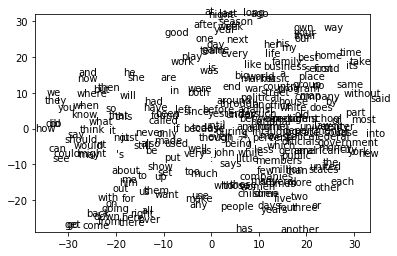
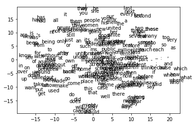
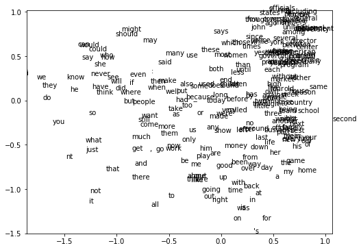
Compared with the second tsne GLoVE plot which has embedded dimension of 256, the first tsne plot has 250 embedded dimension, converges with similar 110 iterations, and has smaller error of about 0.633. The first model trains much slower than GLoVE model, while this tsne graph has more distinguishable clusters, which classifies better than GLoVE model. Some example cluster of words in the first model are: (“has”, “have”, “had”), (“might”, “will”, “would”, “should”, “can”, “may”, “could”), while the second model using GLoVE groups “see” and “say” with “would”, “have” with “called”. The first model with neural net has more precise and clear classification result than the second model.
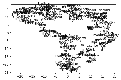
For the third plot, it plots the 2d GLoVE model without tsne, while the fourth plot represents the same model with tsne, converges around 110 iteration with about 0.304 error. Compared with the third plot, the ourth plot with tsne has better clustering, while the third plot is more dispersed and distracted.
tsne_plot_representation(trained_model)
(250, 16)
Preprocessing the data using PCA...
Computing pairwise distances...
Computing P-values for point  0  of  250 ...
Mean value of sigma:  1.0810407640085655
Iteration  10 : error is  13.904534336872707
Iteration  20 : error is  13.649706568082056
...
Iteration  100 : error is  14.403181497189895
Iteration  110 : error is  1.7822399276522192
Iteration  120 : error is  1.3267981771003918
Iteration  130 : error is  1.0994066587715356
Iteration  140 : error is  0.9820645964050435
Iteration  150 : error is  0.8893447064598181
Iteration  160 : error is  0.8501889895414241
Iteration  170 : error is  0.7967478450970407
...
Iteration  910 : error is  0.6337974076653053
Iteration  920 : error is  0.6337973914251336
Iteration  930 : error is  0.6337973768656655
Iteration  940 : error is  0.6337973643741731
Iteration  950 : error is  0.6337973537264191
Iteration  960 : error is  0.6337973444924512
Iteration  970 : error is  0.6337973367838915
Iteration  980 : error is  0.6337973301302106
Iteration  990 : error is  0.6337973244539044
Iteration  1000 : error is  0.6337973197804718
tsne_plot_GLoVE_representation(W_final, b_final)
Preprocessing the data using PCA...
Computing pairwise distances...
Computing P-values for point  0  of  250 ...


/usr/local/lib/python3.6/dist-packages/ipykernel_launcher.py:64: ComplexWarning: Casting complex values to real discards the imaginary part


Mean value of sigma:  0.7414499269370552
Iteration  10 : error is  17.112574187692882
...
Iteration  100 : error is  17.276058343878077
Iteration  110 : error is  2.445460592164862
Iteration  120 : error is  1.7831495425683555
Iteration  130 : error is  1.514816424123761
Iteration  140 : error is  1.408098339641312
...
Iteration  990 : error is  1.1293082792737912
Iteration  1000 : error is  1.1293001798713274

plot_2d_GLoVE_representation(W_final_2d, b_final_2d)
tsne_plot_GLoVE_representation(W_final_2d, b_final_2d)
Preprocessing the data using PCA...
Computing pairwise distances...
Computing P-values for point  0  of  250 ...
Mean value of sigma:  0.23915790027001896
Iteration  10 : error is  12.573822139331822
Iteration  20 : error is  10.52761808422471
...
Iteration  100 : error is  10.378539324143624
Iteration  110 : error is  0.8264687306050834
Iteration  120 : error is  0.5160751571468272
Iteration  130 : error is  0.4342438805667565
Iteration  140 : error is  0.39366570658201167
...
Iteration  980 : error is  0.3044384562592181
Iteration  990 : error is  0.3044384217150869
Iteration  1000 : error is  0.3044383911881474

- As we can see, “new” and “york” are not close together, which is also as expected, because if two words close together, this means that the similarity between two words are very large. While “new” and “york” have very different meanings and nature in language, and should not be categorized into the same group.
print(trained_model.word_distance("new", "york"))
print(trained_model.display_nearest_words("new"))
print(trained_model.display_nearest_words("york"))
3.548393385127713
old: 2.3600505246264323
white: 2.4383030498943365
back: 2.5759303604425643
american: 2.6466202075516416
such: 2.6599246057735786
own: 2.6878098904671783
political: 2.701124031526305
national: 2.7494668874744193
several: 2.7643670072967392
federal: 2.8155523660546993
None
public: 0.9048826050086719
music: 0.9105096376369168
university: 0.9309985183745197
city: 0.9640999583181336
department: 0.9810341593819769
ms.: 0.985606172603071
john: 1.0174907854088202
school: 1.035702631398839
general: 1.0443388378683818
team: 1.0641153998658832
None
- Comparing (“goverment”, “political”) and (“government”, “university”), “government” is more close to “university” rather than “political”. This is plausible, because both of the government and university are noun in a sentance, while political is subjective.
print(trained_model.word_distance("government", "political"))
print(trained_model.word_distance("government", "university"))
1.4021420047033426
0.9350013818643479
Looks nice huh? Stay sharp! 😎