
Convolution Neural Network Part 1
Introduction
This project works with Convolutional Neural Networks and exploring its applications. We will mainly focus on two famous tasks:
- Image Colorization: given a greyscale image, we need to predict its color in each pixel
- difficulties: ill-posed problem – multiple equally valid colorings
- dataset: CIFAR-10 contains 60000 32x32 color images in 10 classes, with 6000 images per class, where 50000 are training images, and 10000 are test images. The 10 classes are horse, automobile, bird, cat, deer, dog, frog, horse, ship, and truck. Our main focus in the horse class
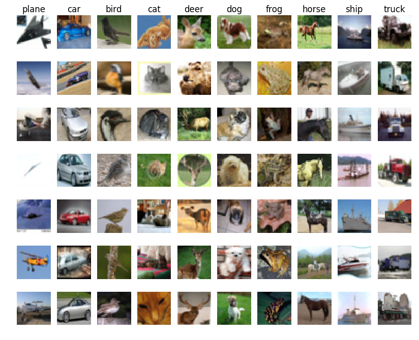
CIFAR-10 Dataset


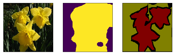
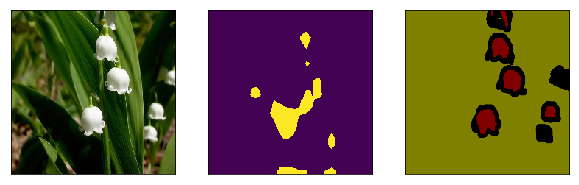
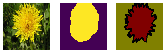
- Semantic Segmentation: cluster areas of an image which belongs to the same object/label, and color with the same color section; We will implement semantic segmentation elaborately in CNN-Part2
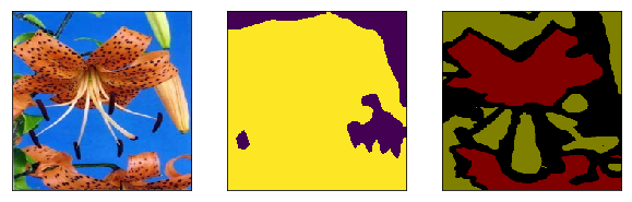
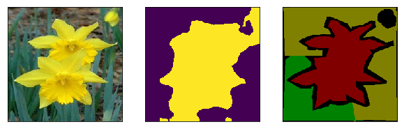
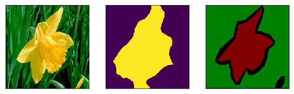
- dataset: Oxford 17 Flowers Dataset 17 categories of flowers with 80 images in each set
- approach: Using Microsoft COCO Dataset, deeplabv3 especially as a finetuning base, and perform semantic segmentation

17 Flowers Dataset
Task 1: Colorization Classification
We will select a subset of 24 colors and frame colorization as a pixel-wise classification problem, where we label each pixel with one of 24 colors. The 24 colors are selected using k-means clustering over colours, and selecting cluster centers
The cluster centers are provided in link, which was downloaded by the helper functions above. For simplicity, we will measure distance in RGB space. This is not ideal and can be improved later.
PS: You can jump to Model section first to get the idea in machine learning since I have already got python dirty work covered for you 😛
Data Handeling
Helper Functions
import os
from six.moves.urllib.request import urlretrieve
import tarfile
import numpy as np
import pickle
import sys
from PIL import Image


def get_file(fname,
             origin,
             untar=False,
             extract=False,
             archive_format='auto',
             cache_dir='data'):
    datadir = os.path.join(cache_dir)
    if not os.path.exists(datadir):
        os.makedirs(datadir)

    if untar:
        untar_fpath = os.path.join(datadir, fname)
        fpath = untar_fpath + '.tar.gz'
    else:
        fpath = os.path.join(datadir, fname)

    print('File path: %s' % fpath)
    if not os.path.exists(fpath):
        print('Downloading data from', origin)

        error_msg = 'URL fetch failure on {}: {} -- {}'
        try:
            try:
                urlretrieve(origin, fpath)
            except URLError as e:
                raise Exception(error_msg.format(origin, e.errno, e.reason))
            except HTTPError as e:
                raise Exception(error_msg.format(origin, e.code, e.msg))
        except (Exception, KeyboardInterrupt) as e:
            if os.path.exists(fpath):
                os.remove(fpath)
            raise

    if untar:
        if not os.path.exists(untar_fpath):
            print('Extracting file.')
            with tarfile.open(fpath) as archive:
                archive.extractall(datadir)
        return untar_fpath

    if extract:
        _extract_archive(fpath, datadir, archive_format)

    return fpath

def load_batch(fpath, label_key='labels'):
    """Internal utility for parsing CIFAR data.
    # Arguments
        fpath: path the file to parse.
        label_key: key for label data in the retrieve
            dictionary.
    # Returns
        A tuple `(data, labels)`.
    """
    f = open(fpath, 'rb')
    if sys.version_info < (3,):
        d = pickle.load(f)
    else:
        d = pickle.load(f, encoding='bytes')
        # decode utf8
        d_decoded = {}
        for k, v in d.items():
            d_decoded[k.decode('utf8')] = v
        d = d_decoded
    f.close()
    data = d['data']
    labels = d[label_key]

    data = data.reshape(data.shape[0], 3, 32, 32)
    return data, labels

def load_cifar10(transpose=False):
    """Loads CIFAR10 dataset.
    # Returns
        Tuple of Numpy arrays: `(x_train, y_train), (x_test, y_test)`.
    """
    dirname = 'cifar-10-batches-py'
    origin = 'http://www.cs.toronto.edu/~kriz/cifar-10-python.tar.gz'
    path = get_file(dirname, origin=origin, untar=True)

    num_train_samples = 50000

    x_train = np.zeros((num_train_samples, 3, 32, 32), dtype='uint8')
    y_train = np.zeros((num_train_samples,), dtype='uint8')

    for i in range(1, 6):
        fpath = os.path.join(path, 'data_batch_' + str(i))
        data, labels = load_batch(fpath)
        x_train[(i - 1) * 10000: i * 10000, :, :, :] = data
        y_train[(i - 1) * 10000: i * 10000] = labels

    fpath = os.path.join(path, 'test_batch')
    x_test, y_test = load_batch(fpath)

    y_train = np.reshape(y_train, (len(y_train), 1))
    y_test = np.reshape(y_test, (len(y_test), 1))

    if transpose:
        x_train = x_train.transpose(0, 2, 3, 1)
        x_test = x_test.transpose(0, 2, 3, 1)
    return (x_train, y_train), (x_test, y_test)
Load Data
The below code may take a few minutes to load the data
# Download cluster centers for k-means over colours
colours_fpath = get_file(fname='colours',
                         origin='http://www.cs.toronto.edu/~jba/kmeans_colour_a2.tar.gz',
                         untar=True)
# Download CIFAR dataset
m = load_cifar10()
(x_train, y_train), (x_test, y_test) = m

# 7 is horse category
indices = [i for i, x in enumerate(y_train) if x == [7]]

# visualize horse data in grey scale
im = Image.fromarray(x_train[indices[0]][0])
im.save('test1.png')


Utility Functions
Helper Code
"""
Colourization of CIFAR-10 Horses via classification.
"""
from __future__ import print_function
import argparse
import math
import numpy as np
import numpy.random as npr
import scipy.misc
import time
import torch
import torch.nn as nn
import torch.nn.functional as F
from torch.autograd import Variable
import matplotlib
import matplotlib.pyplot as plt


#from load_data import load_cifar10

HORSE_CATEGORY = 7
Data Processing
def get_rgb_cat(xs, colours):
    """
    Get colour categories given RGB values. This function doesn't
    actually do the work, instead it splits the work into smaller
    chunks that can fit into memory, and calls helper function
    _get_rgb_cat

    Args:
      xs: float numpy array of RGB images in [B, C, H, W] format
      colours: numpy array of colour categories and their RGB values
    Returns:
      result: int numpy array of shape [B, 1, H, W]
    """
    if np.shape(xs)[0] < 100:
        return _get_rgb_cat(xs)
    batch_size = 100
    nexts = []
    for i in range(0, np.shape(xs)[0], batch_size):
        next = _get_rgb_cat(xs[i:i+batch_size,:,:,:], colours)
        nexts.append(next)
    result = np.concatenate(nexts, axis=0)
    return result

def _get_rgb_cat(xs, colours):
    """
    Get colour categories given RGB values. This is done by choosing
    the colour in `colours` that is the closest (in RGB space) to
    each point in the image `xs`. This function is a little memory
    intensive, and so the size of `xs` should not be too large.

    Args:
      xs: float numpy array of RGB images in [B, C, H, W] format
      colours: numpy array of colour categories and their RGB values
    Returns:
      result: int numpy array of shape [B, 1, H, W]
    """
    num_colours = np.shape(colours)[0]
    xs = np.expand_dims(xs, 0)
    cs = np.reshape(colours, [num_colours,1,3,1,1])
    dists = np.linalg.norm(xs-cs, axis=2) # 2 = colour axis
    cat = np.argmin(dists, axis=0)
    cat = np.expand_dims(cat, axis=1)
    return cat

def get_cat_rgb(cats, colours):
    """
    Get RGB colours given the colour categories

    Args:
      cats: integer numpy array of colour categories
      colours: numpy array of colour categories and their RGB values
    Returns:
      numpy tensor of RGB colours
    """
    return colours[cats]

def process(xs, ys, max_pixel=256.0, downsize_input=False):
    """
    Pre-process CIFAR10 images by taking only the horse category,
    shuffling, and have colour values be bound between 0 and 1

    Args:
      xs: the colour RGB pixel values
      ys: the category labels
      max_pixel: maximum pixel value in the original data
    Returns:
      xs: value normalized and shuffled colour images
      grey: greyscale images, also normalized so values are between 0 and 1
    """
    xs = xs / max_pixel
    xs = xs[np.where(ys == HORSE_CATEGORY)[0], :, :, :]
    npr.shuffle(xs)

    grey = np.mean(xs, axis=1, keepdims=True)

    if downsize_input:
      downsize_module = nn.Sequential(nn.AvgPool2d(2),
                               nn.AvgPool2d(2),
                               nn.Upsample(scale_factor=2),
                               nn.Upsample(scale_factor=2))
      xs_downsized = downsize_module.forward(torch.from_numpy(xs).float())
      xs_downsized = xs_downsized.data.numpy()
      return (xs, xs_downsized)
    else:
      return (xs, grey)


def get_batch(x, y, batch_size):
    '''
    Generated that yields batches of data

    Args:
      x: input values
      y: output values
      batch_size: size of each batch
    Yields:
      batch_x: a batch of inputs of size at most batch_size
      batch_y: a batch of outputs of size at most batch_size
    '''
    N = np.shape(x)[0]
    assert N == np.shape(y)[0]
    for i in range(0, N, batch_size):
        batch_x = x[i:i+batch_size, :,:,:]
        batch_y = y[i:i+batch_size, :,:,:]
        yield (batch_x, batch_y)
Torch Helper Function
def get_torch_vars(xs, ys, gpu=False):
    """
    Helper function to convert numpy arrays to pytorch tensors.
    If GPU is used, move the tensors to GPU.

    Args:
      xs (float numpy tenosor): greyscale input
      ys (int numpy tenosor): categorical labels
      gpu (bool): whether to move pytorch tensor to GPU
    Returns:
      Variable(xs), Variable(ys)
    """
    xs = torch.from_numpy(xs).float()
    ys = torch.from_numpy(ys).long()
    if gpu:
        xs = xs.cuda()
        ys = ys.cuda()
    return Variable(xs), Variable(ys)

def compute_loss(criterion, outputs, labels, batch_size, num_colours):
    """
    Helper function to compute the loss. Since this is a pixelwise
    prediction task we need to reshape the output and ground truth
    tensors into a 2D tensor before passing it in to the loss criteron.

    Args:
      criterion: pytorch loss criterion
      outputs (pytorch tensor): predicted labels from the model
      labels (pytorch tensor): ground truth labels
      batch_size (int): batch size used for training
      num_colours (int): number of colour categories
    Returns:
      pytorch tensor for loss
    """

    loss_out = outputs.transpose(1,3) \
                      .contiguous() \
                      .view([batch_size*32*32, num_colours])
    loss_lab = labels.transpose(1,3) \
                      .contiguous() \
                      .view([batch_size*32*32])
    return criterion(loss_out, loss_lab)

def run_validation_step(cnn, criterion, test_grey, test_rgb_cat, batch_size,
                        colours, plotpath=None, visualize=True, downsize_input=False):
    correct = 0.0
    total = 0.0
    losses = []
    num_colours = np.shape(colours)[0]
    for i, (xs, ys) in enumerate(get_batch(test_grey,
                                           test_rgb_cat,
                                           batch_size)):
        images, labels = get_torch_vars(xs, ys, args.gpu)
        outputs = cnn(images)

        val_loss = compute_loss(criterion,
                                outputs,
                                labels,
                                batch_size=args.batch_size,
                                num_colours=num_colours)
        losses.append(val_loss.data.item())

        _, predicted = torch.max(outputs.data, 1, keepdim=True)
        total += labels.size(0) * 32 * 32
        correct += (predicted == labels.data).sum()

    if plotpath: # only plot if a path is provided
        plot(xs, ys, predicted.cpu().numpy(), colours,
             plotpath, visualize=visualize, compare_bilinear=downsize_input)

    val_loss = np.mean(losses)
    val_acc = 100 * correct / total
    return val_loss, val_acc
Visualizations
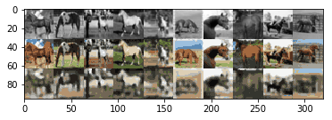
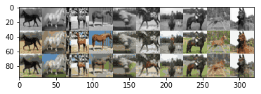
def plot(input, gtlabel, output, colours, path, visualize, compare_bilinear=False):
    """
    Generate png plots of input, ground truth, and outputs

    Args:
      input: the greyscale input to the colourization CNN
      gtlabel: the grouth truth categories for each pixel
      output: the predicted categories for each pixel
      colours: numpy array of colour categories and their RGB values
      path: output path
      visualize: display the figures inline or save the figures in path
    """
    grey = np.transpose(input[:10,:,:,:], [0,2,3,1])
    gtcolor = get_cat_rgb(gtlabel[:10,0,:,:], colours)
    predcolor = get_cat_rgb(output[:10,0,:,:], colours)

    img_stack = [
      np.hstack(np.tile(grey, [1,1,1,3])),
      np.hstack(gtcolor),
      np.hstack(predcolor)]

    if compare_bilinear:
      downsize_module = nn.Sequential(nn.AvgPool2d(2),
                                 nn.AvgPool2d(2),
                                 nn.Upsample(scale_factor=2, mode='bilinear'),
                                 nn.Upsample(scale_factor=2, mode='bilinear'))
      gt_input = np.transpose(gtcolor, [0, 3, 1, 2,])
      color_bilinear = downsize_module.forward(torch.from_numpy(gt_input).float())
      color_bilinear = np.transpose(color_bilinear.data.numpy(), [0, 2, 3, 1])
      img_stack = [
        np.hstack(np.transpose(input[:10,:,:,:], [0,2,3,1])),
        np.hstack(gtcolor),
        np.hstack(predcolor),
        np.hstack(color_bilinear)]
    img = np.vstack(img_stack)

    plt.grid('off')
    plt.imshow(img, vmin=0., vmax=1.)
    if visualize:
      plt.show()
    else:
      plt.savefig(path)

def toimage(img, cmin, cmax):
    return Image.fromarray((img.clip(cmin, cmax)*255).astype(np.uint8))

def plot_activation(args, cnn):
    # LOAD THE COLOURS CATEGORIES
    colours = np.load(args.colours, allow_pickle=True)[0]
    num_colours = np.shape(colours)[0]

    (x_train, y_train), (x_test, y_test) = load_cifar10()
    test_rgb, test_grey = process(x_test, y_test, downsize_input = args.downsize_input)
    test_rgb_cat = get_rgb_cat(test_rgb, colours)

    # Take the idnex of the test image
    id = args.index
    outdir = "outputs/" + args.experiment_name + '/act' + str(id)
    if not os.path.exists(outdir):
      os.makedirs(outdir)
    images, labels = get_torch_vars(np.expand_dims(test_grey[id], 0),
                                    np.expand_dims(test_rgb_cat[id], 0))
    cnn.cpu()
    outputs = cnn(images)
    _, predicted = torch.max(outputs.data, 1, keepdim=True)
    predcolor = get_cat_rgb(predicted.cpu().numpy()[0,0,:,:], colours)
    img = predcolor
    toimage(predcolor, cmin=0, cmax=1) \
            .save(os.path.join(outdir, "output_%d.png" % id))

    if not args.downsize_input:
      img = np.tile(np.transpose(test_grey[id], [1,2,0]), [1,1,3])
    else:
      img = np.transpose(test_grey[id], [1,2,0])
    toimage(img, cmin=0, cmax=1) \
            .save(os.path.join(outdir, "input_%d.png" % id))

    img = np.transpose(test_rgb[id], [1,2,0])
    toimage(img, cmin=0, cmax=1) \
            .save(os.path.join(outdir, "input_%d_gt.png" % id))


    def add_border(img):
        return np.pad(img, 1, "constant", constant_values=1.0)

    def draw_activations(path, activation, imgwidth=4):
        img = np.vstack([
            np.hstack([
                add_border(filter) for filter in
                activation[i*imgwidth:(i+1)*imgwidth,:,:]])
            for i in range(activation.shape[0] // imgwidth)])
        scipy.misc.imsave(path, img)


    for i, tensor in enumerate([cnn.out1, cnn.out2, cnn.out3, cnn.out4, cnn.out5]):
        draw_activations(
            os.path.join(outdir, "conv%d_out_%d.png" % (i+1, id)),
            tensor.data.cpu().numpy()[0])
    print("visualization results are saved to %s"%outdir)
Trainings Loop
class AttrDict(dict):
def __init__(self, *args, **kwargs):
super(AttrDict, self).__init__(*args, **kwargs)
self.__dict__ = self
def train(args, cnn=None):
# Set the maximum number of threads to prevent crash in Teaching Labs
#TODO: necessary?
torch.set_num_threads(5)
# Numpy random seed
npr.seed(args.seed)
# Save directory
save_dir = "outputs/" + args.experiment_name
# LOAD THE COLOURS CATEGORIES
colours = np.load(args.colours, allow_pickle=True)[0]
num_colours = np.shape(colours)[0]
# INPUT CHANNEL
num_in_channels = 1 if not args.downsize_input else 3
# LOAD THE MODEL
if cnn is None:
if args.model == "CNN":
cnn = CNN(args.kernel, args.num_filters, num_colours, num_in_channels)
elif args.model == "UNet":
cnn = UNet(args.kernel, args.num_filters, num_colours, num_in_channels)
# LOSS FUNCTION
criterion = nn.CrossEntropyLoss()
optimizer = torch.optim.Adam(cnn.parameters(), lr=args.learn_rate)
# DATA
print("Loading data...")
(x_train, y_train), (x_test, y_test) = load_cifar10()
print("Transforming data...")
train_rgb, train_grey = process(x_train, y_train, downsize_input = args.downsize_input)
train_rgb_cat = get_rgb_cat(train_rgb, colours)
test_rgb, test_grey = process(x_test, y_test, downsize_input = args.downsize_input)
test_rgb_cat = get_rgb_cat(test_rgb, colours)
# Create the outputs folder if not created already
if not os.path.exists(save_dir):
os.makedirs(save_dir)
print("Beginning training ...")
if args.gpu: cnn.cuda()
start = time.time()
train_losses = []
valid_losses = []
valid_accs = []
for epoch in range(args.epochs):
# Train the Model
cnn.train() # Change model to 'train' mode
losses = []
for i, (xs, ys) in enumerate(get_batch(train_grey,
train_rgb_cat,
args.batch_size)):
images, labels = get_torch_vars(xs, ys, args.gpu)
# Forward + Backward + Optimize
optimizer.zero_grad()
outputs = cnn(images)
loss = compute_loss(criterion,
outputs,
labels,
batch_size=args.batch_size,
num_colours=num_colours)
loss.backward()
optimizer.step()
losses.append(loss.data.item())
# plot training images
if args.plot:
_, predicted = torch.max(outputs.data, 1, keepdim=True)
plot(xs, ys, predicted.cpu().numpy(), colours,
save_dir+'/train_%d.png' % epoch,
args.visualize,
args.downsize_input)
# plot training images
avg_loss = np.mean(losses)
train_losses.append(avg_loss)
time_elapsed = time.time() - start
print('Epoch [%d/%d], Loss: %.4f, Time (s): %d' % (
epoch+1, args.epochs, avg_loss, time_elapsed))
# Evaluate the model
cnn.eval() # Change model to 'eval' mode (BN uses moving mean/var).
val_loss, val_acc = run_validation_step(cnn,
criterion,
test_grey,
test_rgb_cat,
args.batch_size,
colours,
save_dir+'/test_%d.png' % epoch,
args.visualize,
args.downsize_input)
time_elapsed = time.time() - start
valid_losses.append(val_loss)
valid_accs.append(val_acc)
print('Epoch [%d/%d], Val Loss: %.4f, Val Acc: %.1f%%, Time(s): %.2f' % (
epoch+1, args.epochs, val_loss, val_acc, time_elapsed))
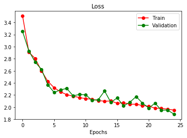
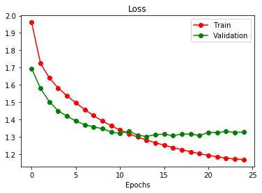
# Plot training curve
plt.figure()
plt.plot(train_losses, "ro-", label="Train")
plt.plot(valid_losses, "go-", label="Validation")
plt.legend()
plt.title("Loss")
plt.xlabel("Epochs")
plt.savefig(save_dir+"/training_curve.png")
if args.checkpoint:
print('Saving model...')
torch.save(cnn.state_dict(), args.checkpoint)
return cnn
Model !!!!!!!
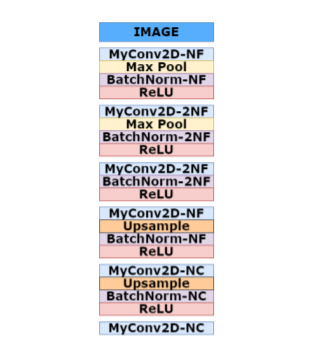 In the diagram, we denote the number of filters as NF. Further layers double the number of filters, denoted as 2NF. In the final layers, the number of filters will be equivalent to the number of colour classes, denoted as NC. Consequently, your constructed neural network should define the number of input/output layers with respect to the variables
 num_filters and num_colours, as opposed to a constant value.
We will use our own convolution module MyConv2d instead of PyTorch’s nn.Conv2D to better understand its internals.
Each MyConv2d layer should be parameterized as follows:
- The number of channels in the image is defined in
num_in_channels. Use this as the number of input filters for the first convolution. - The number of output filters for each MyConv2d layer is specified after the hyphen.
- The kernel size used in MyConv2d should be specified via the
kernelparameter.
For the remaining operations, you may use the default PyTorch implementations.
The specific modules to use are listed below. If parameters are not otherwise specified, use the default PyTorch parameters.
-
nn.MaxPool2d: Use
kernel_size=2for all layers. -
nn.BatchNorm2d: The number of features is specified after the hyphen in the diagram as a multiple of NF or NC.
-
nn.Upsample: Use
scaling_factor=2for all layers.
We recommend grouping each block of operations (those adjacent without whitespace in the diagram) into nn.Sequential containers.
Grouping up relevant operations will allow for easier implementation of the forward method.
class MyConv2d(nn.Module):
    """
    Our simplified implemented of nn.Conv2d module for 2D convolution
    """
    def __init__(self, in_channels, out_channels, kernel_size, padding=None):
        super(MyConv2d, self).__init__()

        self.in_channels = in_channels
        self.out_channels = out_channels
        self.kernel_size = kernel_size
        if padding is None:
            self.padding = kernel_size // 2
        else:
            self.padding = padding
        self.weight = nn.parameter.Parameter(torch.Tensor(
            out_channels, in_channels, kernel_size, kernel_size))
        self.bias = nn.parameter.Parameter(torch.Tensor(out_channels))
        self.reset_parameters()

    def reset_parameters(self):
        n = self.in_channels * self.kernel_size * self.kernel_size
        stdv = 1. / math.sqrt(n)
        self.weight.data.uniform_(-stdv, stdv)
        self.bias.data.uniform_(-stdv, stdv)

    def forward(self, input):
        return F.conv2d(input, self.weight, self.bias, padding=self.padding)


class CNN(nn.Module):
    def __init__(self, kernel, num_filters, num_colours, num_in_channels):
        super(CNN, self).__init__()
        padding = kernel // 2
        self.downconv1 = nn.Sequential(
            MyConv2d(num_in_channels, num_filters, kernel_size=kernel, padding=padding),
            nn.BatchNorm2d(num_filters),
            nn.ReLU(),
            nn.MaxPool2d(2),)

        self.downconv2 = nn.Sequential(
            MyConv2d(num_filters, num_filters*2, kernel_size=kernel, padding=padding),
            nn.BatchNorm2d(num_filters*2),
            nn.ReLU(),
            nn.MaxPool2d(2),)

        self.rfconv = nn.Sequential(
            MyConv2d(num_filters*2, num_filters*2, kernel_size=kernel, padding=padding),
            nn.BatchNorm2d(num_filters*2),
            nn.ReLU())

        self.upconv1 = nn.Sequential(
            MyConv2d(num_filters*2, num_filters, kernel_size=kernel, padding=padding),
            nn.BatchNorm2d(num_filters),
            nn.ReLU(),
            nn.Upsample(scale_factor=2),)

        self.upconv2 = nn.Sequential(
            MyConv2d(num_filters, num_colours, kernel_size=kernel, padding=padding),
            nn.BatchNorm2d(num_colours),
            nn.ReLU(),
            nn.Upsample(scale_factor=2),)

        self.finalconv = MyConv2d(num_colours, num_colours, kernel_size=kernel)

    def forward(self, x):
        self.out1 = self.downconv1(x)
        self.out2 = self.downconv2(self.out1)
        self.out3 = self.rfconv(self.out2)
        self.out4 = self.upconv1(self.out3)
        self.out5 = self.upconv2(self.out4)
        self.out_final = self.finalconv(self.out5)
        return self.out_final
Now, we can train the model and generate few results over 25 epoches
args = AttrDict()
args_dict = {
              'gpu':True,
              'valid':False,
              'checkpoint':"",
              'colours':'./data/colours/colour_kmeans24_cat7.npy',
              'model':"CNN",
              'kernel':3,
              'num_filters':32,
              'learn_rate':0.3,
              'batch_size':100,
              'epochs':25,
              'seed':0,
              'plot':True,
              'experiment_name': 'colourization_cnn',
              'visualize': False,
              'downsize_input':False,
}
args.update(args_dict)
cnn = train(args)
We can see that the colorization is gnerealized with proceding training, but poorly on result.
IMPROVEMENTS with Skip Connections

We will introduce skip connections to our previous model. A skip connection in a neural network is a connection which skips one or more layer and connects to a later layer.
we will be adding a skip connection from the first layer to the last, second layer to the second last, etc. That is, the final convolution should have both the output of the previous layer and the initial greyscale input as input. This type of skip-connection is introduced by Ronneberger et al.[2015], and is called a ”UNet”.
class UNet(nn.Module):
    def __init__(self, kernel, num_filters, num_colours, num_in_channels):
        super(UNet, self).__init__()
        padding = kernel // 2
        self.model1 = nn.Sequential(
            MyConv2d(num_in_channels, num_filters, kernel, padding= padding),
            nn.MaxPool2d(2),
            nn.BatchNorm2d(num_filters),
            nn.ReLU()
        )
        self.model2 = nn.Sequential(
            MyConv2d(num_filters, num_filters*2, kernel, padding= padding),
            nn.MaxPool2d(2),
            nn.BatchNorm2d(2*num_filters),
            nn.ReLU()
        )
        self.model3 = nn.Sequential(
            MyConv2d(num_filters*2, num_filters*2, kernel, padding= padding),
            nn.BatchNorm2d(num_filters*2),
            nn.ReLU()
        )
        self.model4 = nn.Sequential(
            MyConv2d(num_filters*4, num_filters, kernel, padding= padding),
            nn.Upsample(scale_factor=2),
            nn.BatchNorm2d(num_filters),
            nn.ReLU()
        )
        self.model5 = nn.Sequential(
            MyConv2d(num_filters*2, num_colours, kernel, padding= padding),
            nn.Upsample(scale_factor=2),
            nn.BatchNorm2d(num_colours),
            nn.ReLU()
        )
        self.model6 = nn.Sequential(
            MyConv2d(num_colours+num_in_channels, num_colours, kernel, padding= padding)
        )

    def forward(self, x):
        self.layer1 = self.model1(x)
        self.layer2 = self.model2(self.layer1)
        self.layer3 = self.model3(self.layer2)
        self.layer4 = self.model4(torch.cat((self.layer3, self.layer2), dim=1))
        self.layer5 = self.model5(torch.cat((self.layer4, self.layer1), dim=1))
        self.layer6 = self.model6(torch.cat((self.layer5, x), dim=1))
        return self.layer6
Then we train the improved Unet with another 25 epoches
args = AttrDict()
args_dict = {
              'gpu':True,
              'valid':False,
              'checkpoint':"",
              'colours':'./data/colours/colour_kmeans24_cat7.npy',
              'model':"UNet",
              'kernel':3,
              'num_filters':32,
              'learn_rate':0.001,
              'batch_size':10,
              'epochs':25,
              'seed':0,
              'plot':True,
              'experiment_name': 'colourization_unet',
              'visualize': False,
              'downsize_input':False,
}
args.update(args_dict)
unet_cnn = train(args)
The result is much better with smaller errors, better generalizations and coloring
Continues …

Now we have our colorization task settles, go to the next part to see the Semantic Segmentation